The tutorial explains the essentials of the table format, shows how to make a table in Excel and leverage its powerful features.
At the surface, an Excel table just sounds like a way to organize data. In truth, this generic name covers a ton of useful features. Tables containing hundreds or even thousands of rows and columns can be instantly recalculated and totaled, sorted and filtered, updated with new information and reformatted, summarized with pivot tables and exported.
Excel table
You might be under the impression that the data in your worksheet is already in a table simply because it's organized in rows and columns. However, the data in a tabular format is not a true "table" unless you've specifically made it such.
Excel table is a special object that works as a whole and allows you to manage the table's contents independently from the rest of the worksheet data.
The screenshot below contrasts a regular range and the table format:

The most obvious difference is that the table is styled. However, an Excel table is far more than a range of formatted data with headings. There are many powerful features inside:
- Excel tables are dynamic by nature, meaning they expand and contract automatically as you add or remove rows and columns.
- Integrated sort and filter options; visual filtering with slicers.
- Easy formatting with inbuilt table styles.
- Column headings remain visible while scrolling.
- Quick totals allow you to sum and count data as well as find average, min or max value in a click.
- Calculated columns allow you to compute an entire column by entering a formula in one cell.
- Easy-to-read formulas due to a special syntax that uses table and column names rather than cell references.
- Dynamic charts adjust automatically as you add or remove data in a table.
For more information, please see 10 most useful features of Excel tables.
How to create a table in Excel
With the source data organized in rows and columns, carry out the below steps to covert a range of cells into a table:
- Select any cell within your data set.
- On the Insert tab, in the Tables group, click the Table button or press the Ctrl + T shortcut.
- The Create Table dialog box appears with all the data selected for you automatically; you can adjust the range if needed. If you want the first row of data to become the table headers, make sure the My table has headers box is selected.
- Click OK.
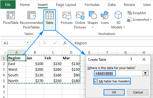
As the result, Excel converts your range of data into a true table with the default style:

Many wonderful features are now just a click away and, in a moment, you will learn how to use them. But first, we'll look at how to make a table with a specific style.
Tips and notes:
- Prepare and clean your data before creating a table: remove blank rows, give each column a unique meaningful name, and make sure each row contains information about one record.
- When a table is inserted, Excel retains all formatting that you currently have. For best results, you may want to remove some of the existing formatting, e.g. background colors, so it does not conflict with a table style.
- You are not limited to just one table per sheet, you can have as many as needed. For better readability, it stands to reason to insert at least one blank row and one blank column between a table and other data.
How to make a table with a selected style
The previous example showed the fastest way to create a table in Excel, but it always uses the default style. To draw a table with the style of your choosing, perform these steps:
- Select any cell in your data set.
- On the Home tab, in the Styles group, click Format as Table.
- In the gallery, click on the style you want to use.
- In the Create Table dialog box, adjust the range if necessary, check the My table has headers box, and click OK.
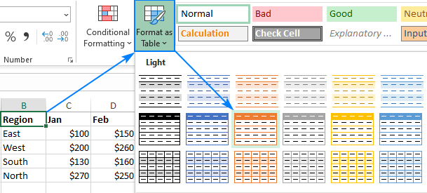
Tip. To apply the selected style and remove all existing formatting, right-click the style and choose Apply and Clear Formatting from the context menu.
How to name a table in Excel
Every time you make a table in Excel, it automatically gets a default name such asTable1, Table2, etc. When you deal with multiple tables, changing the default names to something more meaningful and descriptive can make your work a lot easier.
To rename a table, just do the following:
- Select any cell in the table.
- On the Table Design tab, in the Properties group, select the existing name in the Table Name box, and overwrite it with a new one.
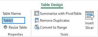
Tip. To view the names of all tables in the current workbook, press Ctrl + F3 to open the Name Manager.
How to use tables in Excel
Excel tables have many awesome features that simply calculating, manipulating and updating data in your worksheets. Most of these features are intuitive and straightforward. Below you will find a quick overview of the most important ones.
How to filter a table in Excel
All tables get the auto-filter capabilities by default. To filter the table's data, this is what you need to do:
- Click the drop-down arrow in the column header.
- Uncheck the boxes next to the data you want to filter out. Or uncheck the Select All box to deselect all the data, and then check the boxes next to the data you want to show.
- Optionally, you can use the Filter by Color and Text Filters options where appropriate.
- Click OK.
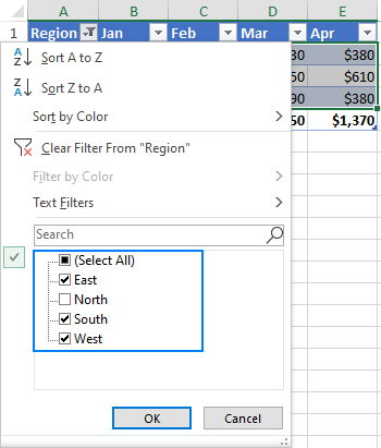
If you don't need the auto-filter feature, you can remove the arrows by unchecking the Filter Button box on the Design tab, in the Table Style Options group. Or you can toggle the filter buttons on and off with the Ctrl + Shift + L shortcut.

Additionally, you can create a visual filter for your table by adding a slicer. For this, click Insert Slicer on the Table Design tab, in the Tools group.

How to sort a table in Excel
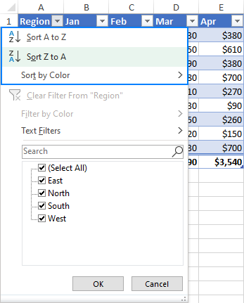
To sort a table by a specific column, just click the drop-down arrow in the heading cell, and pick the required sorting option:
Excel table formulas
For calculating the table data, Excel uses a special formula syntax called structured references. Compared to regular formulas, they have a number of advantages:
- Easy-to-create. Simply select the table's data when making a formula, and Excel will build a structured reference for you automatically.
- Easy-to-read. Structured references refer to the table parts by name, which makes formulas easier to understand.
- Auto-filled. To perform the same calculation in each row, enter a formula in any single cell, and it will be immediately copied throughout the column.
- Changed automatically. When you modify a formula anywhere in a column, the other formulas in the same column will change accordingly.
- Updated automatically. Every time the table is resized or the columns renamed, structured references update dynamically.
The screenshot below shows an example of a structured reference that sums data in each row:

Sum table columns
Another great feature of an Excel table is the ability to summarize data without formulas. This option is called Total Row.
To sum a table's data, this is what you need to do:
- Select any cell in the table.
- On the Design tab, in the Table Style Options group, put a tick mark in the Total Row box.
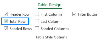
The Total row is inserted at the bottom of the table and shows the total in the last column:

To sum data in other columns, click in the Total cell, then click the drop-down arrow and choose the SUM function. To calculate data in a different way, e.g. count or average, select the corresponding function.
Whatever operation you choose, Excel would use the SUBTOTAL function that calculates data only in visible rows:

Tip. To toggle the Total Row on and off, use the Ctrl + Shift + T shortcut.
How to extend a table in Excel
When you type anything in an adjacent cell, an Excel table expands automatically to include the new data. Combined with structured references, this creates a dynamic range for your formulas without any effort from your side. If you don't mean the new data to be part of the table, press Ctrl + Z. This will undo the table expansion but keep the data that you typed.
You can also extend a table manually by dragging a little handle at the bottom-right corner.

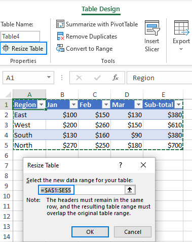
You can also add and remove columns and rows by using the Resize Table command. Here's how:
- Click anywhere in your table.
- On the Design tab, in the Properties group, click Resize Table.
- When the dialog box appears, select the range to be included in the table.
- Click OK.
Excel table styles
Tables are very easily formatted due to a predefined gallery of styles. Additionally, you can create a custom style with your own formatting.
How to change table style
When you insert a table in Excel, the default style is automatically applied to it. To change a table style, do the following:
- Select any cell in the table.
- On the Design tab, in the Table Styles group, click on the style you want to apply. To see all the styles, click the More button in the down-right corner.

Tips:
- To create your own style, please follow these guidelines: How to make a custom table style.
- To change the default table style, right-click the desired style and choose Set as Default. Any new table that you create in the same workbook will now be formatted with the new the default table style.
Apply a table style and remove existing formatting
When you format a table with any predefined style, Excel preserves the formatting you already have. To remove any existing formatting, right-click the style and choose Apply and Clear formatting:

Manage banded rows and columns
To add or remove banded rows and columns as well as apply special formatting for the first or last column, simply tick or untick the corresponding checkbox on the Design tab in the Table Style Options group:

For more information, please see How to alternate row / column colors in Excel.
How to remove table formatting
If you'd like to have all the functionality of an Excel table but do not want any formatting such as banded rows, table borders and the like, you can remove formatting in this way:
- Select any cell within your table.
- On the Design tab, in the Table Styles group, click the More button in the bottom-right corner, and then click Clear underneath the table style templates. Or pick the first style under Light, which is called None.

Note. This method only removes the inbuilt table formatting, your custom formatting is preserved. To remove absolutely all formatting in a table, go to the Home tab > Formats group, and click Clear > Clear formats.
For more information, see How to remove table formatting in Excel.
How to remove table in Excel
Removing a table is as easy as inserting it. To convert a table back to a range, just do the following:
- Right-click any cell in your table, and then click Table> Convert to Range. Or click the Convert to Range button on the Design tab, in the Tools group.
- In the dialog box that appear, click Yes.
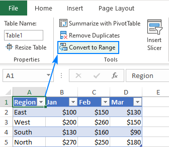
This will remove the table but retain all the data and formatting. To keep only the data, remove table formatting before converting your table to a range.
This is how you create, edit and remove a table in Excel. I thank you for reading and hope to see you on our blog next week!
 by
by
2 comments
My experience over time is that Excel help from https://www.ablebits.com/ and Svetlana Cheusheva is the absolute best. My questions concerns the "Create Table" dialog box. #1 What is the name for the odd-looking arrow control. #2 How is the odd-looking arrow used if one chooses to use it? I thank you in advance for your attention to my questions.
Hi Ald!
Thank you so much for your kind words!
As far as I understand, you are asking about the Collapses Dialog button (a small black upward arrow). This button collapses the current dialog box so you can select a cell or a range of cells on the sheet. After you click it, the button changes to an Expand Dialog icon.