How to make and use a data table in Excel

The tutorial shows how to use data tables for What-If analysis in Excel. Learn how to create a one-variable and two-variable table to see the effects of one or two input values on your formula, and how to set up a data table to evaluate multiple formulas at once.

You have built a complex formula dependent on multiple variables and want to know how changing those inputs changes the results. Instead of testing each variable individually, make a What-if analysis data table and observe all possible outcomes with a quick glance!

• Data table in Excel
• Create one variable data table
• Make two variable data table
• Data table to evaluate multiple formulas
• Excel data tables - 3 things you should know
• Delete a data table in Excel
• Edit data table results
• Recalculate data table manually

What is a data table in Excel?

In Microsoft Excel, a data table is one of the What-If Analysis tools that allows you to try out different input values for formulas and see how changes in those values affect the formulas output.

Data tables are especially useful when a formula depends on several values, and you'd like to experiment with different combinations of inputs and compare the results.

Currently, there exist one variable data table and two variable data table. Although limited to a maximum of two different input cells, a data table enables you to test as many variable values as you want.

How to create a one variable data table in Excel

One variable data table in Excel allows testing a series of values for a single input cell and shows how those values influence the result of a related formula.

To help you better understand this feature, we are going to follow a specific example rather than describing generic steps.

Suppose you are considering depositing your savings in a bank, which pays 5% interest that compounds monthly. To check different options, you've built the following compound interest calculator where:

• B8 contains the FV formula that calculates the closing balance.
• B2 is the variable you want to test (initial investment).

And now, let's do a simple What-If analysis to see what your savings will be in 5 years depending on the amount of your initial investment, ranging from $1,000 to $6,000.

Here are the steps to make a one-variable data table:

1. Enter the variable values either in one column or across one row. In this example, we are going to create a column-oriented data table, so we type our variable values in a column (D3:D8) and leave at least one blank column to the right for the outcomes.
2. Type your formula in the cell one row above and one cell to the right of the variable values (E2 in our case). Or, link this cell to the formula in your original dataset (if you decide to change the formula in the future, you would need to update only one cell). We choose the latter option, and enter this simple formula in E2: =B8
   

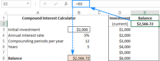
   Tip. If you want to examine the impact of the variable values on other formulas that refer to the same input cell, enter the additional formula(s) to the right of the first formula, as shown in this example.

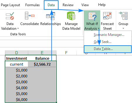
3. Select the data table range, including your formula, variable values cells, and empty cells for the results (D2:E8).
4. Go to the Data tab > Data Tools group, click the What-If Analysis button, and then click Data Table…
   
5. In the Data Table dialog window, click in the Column Input cell box (because our Investment values are in a column), and select the variable cell referenced in your formula. In this example, we select B3 that contains the initial investment value.
   
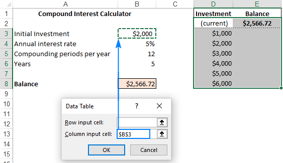
6. Click OK, and Excel will immediately populate the empty cells with outcomes corresponding to the variable value in the same row.
7. Apply the desired number format to the results (Currency in our case), and you are good to go!

Now, you can take a quick look at your one-variable data table, examine the possible balances and choose the optimal deposit size:

Row-oriented data table

The above example shows how to set up a vertical, or column-oriented, data table in Excel. If you prefer a horizontal layout, here's what you need to do:

1. Type the variable values in a row, leaving at least one empty column to the left (for the formula) and one empty row below (for the results). For this example, we enter the variable values in cells F3:J3.
2. Enter the formula in the cell that is one column to the left of your first variable value and one cell below (E4 in our case).
3. Make a data table as discussed above, but enter the input value (B3) in the Row input cell box:
   
4. Click OK, and you will have the following result:
   

How to make a two variable data table in Excel

A two-variable data table shows how various combinations of 2 sets of variable values affect the formula result. In other words, it shows how changing two input values of the same formula changes the output.

The steps to create a two-variable data table in Excel are basically the same as in the above example, except that you enter two ranges of possible input values, one in a row and another in a column.

To see how it works, let's use the same compound interest calculator and examine the effects of the size of the initial investment and the number of years on the balance. To have it done, set up your data table in this way:

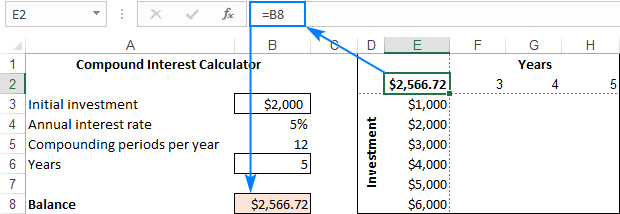
1. Enter your formula in a blank cell or link that cell to your original formula. Make sure you have enough empty columns to the right and empty rows below to accommodate your variable values. As before, we link the cell E2 to the original FV formula that calculates the balance: =B8
2. Type one set of input values below the formula, in the same column (investment values in E3:E8).
3. Enter the other set of variable values to the right of the formula, in the same row (number of years in F2:H2).

   At this point, your two variable data table should look similar to this:
   

4. Select the entire data table range including the formula, the row and column of the variable values, and the cells in which the calculated values will appear. We select the range E2:H8.
5. Create a data table in the already familiar way: Data tab > What-If Analysis button > Data Table…
6. In the Row input cell box, enter the reference to the input cell for the variable values in the row (in this example, it's B6 containing the Years value).
7. In the Column input cell box, enter the reference to the input cell for the variable values in the column (B3 containing the Initial Investment value).
8. Click OK.
   
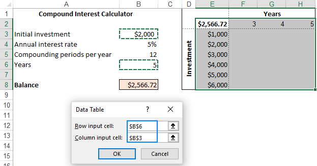
9. Optionally, format the outputs the way you need (by applying the Currency format in our case), and analyze the results:
   

Data table to compare multiple results

If you wish to evaluate more than one formula at the same time, build your data table as shown in the previous examples, and enter the additional formula(s):

• To the right of the first formula in case of a vertical data table organized in columns
• Below the first formula in case of a horizontal data table organized in rows

For the "multi-formula" data table to work correctly, all the formulas should refer to the same input cell.

As an example, let's add one more formula to our one-variable data table to calculate the interest and see how it is affected by the size of the initial investment. Here's what we do:

1. In cell B10, compute the interest with this formula: =B8-B3
2. Arrange the data table's source data like we did earlier: variable values in D3:D8 and E2 linked to B8 (Balance formula).
3. Add one more column to the data table range (column F), and link F2 to B10 (interest formula):
   
4. Select the extended data table range (D2:F8).
5. Open the Data Table dialog box by clicking Data tab > What-If Analysis > Data Table…
6. In the Column Input cell box, supply the input cell (B3), and click OK.

Voilà, you can now observe the effects of your variable values on both formulas:

Data table in Excel - 3 things you should know

To effectively use data tables in Excel, please keep in mind these 3 simple facts:

1. For a data table to be created successfully, the input cell(s) must be on the same sheet as the data table.
2. Microsoft Excel uses the TABLE(row_input_cell, colum_input_cell) function to calculate data table results:
   • In one-variable data table, one of the arguments is omitted, depending on the layout (column-oriented or row-oriented). For example, in our horizontal one-variable data table, the formula is =TABLE(, B3) where B3 is the column input cell.
   • In two-variable data table, both arguments are in place. For example, =TABLE(B6, B3) where B6 is the row input cell and B3 is the column input cell.

   The TABLE function is entered as an array formula. To make sure of this, select any cell with the calculated value, look at the formula bar, and note the {curly brackets} around the formula. However, it is not a normal array formula - you can't type it in the formula bar nor can you edit an existing one. It is just "for show".

3. Because the data table results are calculated with an array formula, the resulting cells cannot be edited individually. You can only edit or delete the entire array of cells as explained below.

How to delete a data table in Excel

As mentioned above, Excel does not allow deleting values in individual cells containing the results. Whenever you try to do this, an error message "Cannot change part of a data table" will show up.

However, you can easily clear the entire array of the resulting values. Here's how:

1. Depending on your needs, select all the data table cells or only the cells with the results.
2. Press the Delete key.

Done! :)

How to edit data table results

Since it is not possible to change part of an array in Excel, you cannot edit individual cells with calculated values. You can only replace all those values with your own one by performing these steps:

1. Select all the resulting cells.
2. Delete the TABLE formula in the formula bar.
3. Type the desired value, and press Ctrl + Enter.

This will insert the same value in all the selected cells:

Once the TABLE formula is gone, the former data table becomes a usual range, and you are free to edit any individual cell normally.

How to recalculate data table manually

If a large data table with multiple variable values and formulas slows down your Excel, you can disable automatic recalculations in that and all other data tables.

For this, go to the Formulas tab > Calculation group, click the Calculation Options button, and then click Automatic Except Data Tables.

This will turn off automatic data table calculations and speed up recalculations of the entire workbook.

To manually recalculate your data table, select its resulting cells, i.e. the cells with TABLE() formulas, and press F9.

This is how you create and use a data table in Excel. To have a closer look at the examples discussed this this tutorial, you are welcome to download our sample Excel Data Tables workbook. I thank you for reading and would be happy to see you again next week!

You may also be interested in

• What-If analysis with Goal Seek in Excel
• Using Excel FORECAST functions with examples
• How to use Solver in Excel: step-by-step with examples
• How to group rows in Excel