When you use different colors to organize your data in Google Sheets, you might find there are no built-in formulas to easily summarize data based on color. To address this, we introduced several custom functions that take into account both the font and background color of cells for basic operations, making it possible for your Google Sheets to sum by color or count cells by color.
You will find these functions among the smart 40+ features of our Power Tools collection or as an individual tool: Function by Color. Both offer a 30-day trial period and two subscription plans: 12-month and lifetime.
How to count colored cells in Google Sheets
Let's take one of the most common tasks with colored cells in a spreadsheet: counting cells that have the same formatting. Say, here I have a list of grades and I want to see how many times each test was passed, i.e. count all green cells in a column:
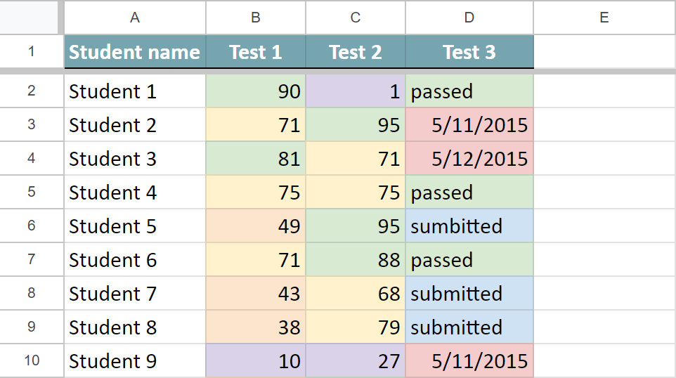
If you're dealing with ranges that include various data types like numbers, text, or dates, consider using the COUNTA function from the Function by Color tool.
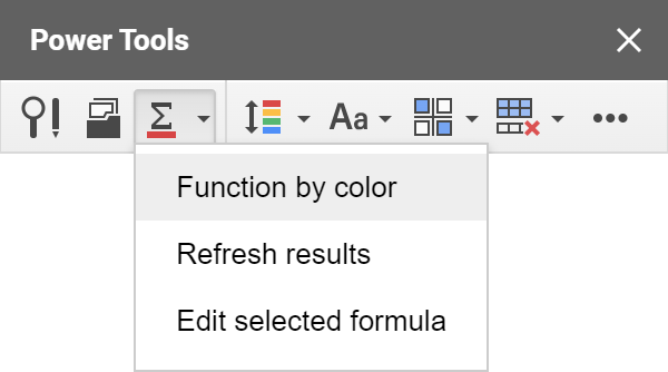
For a start, open the tool to sum by color. In Power Tools, you will see it right on the smart toolbar:
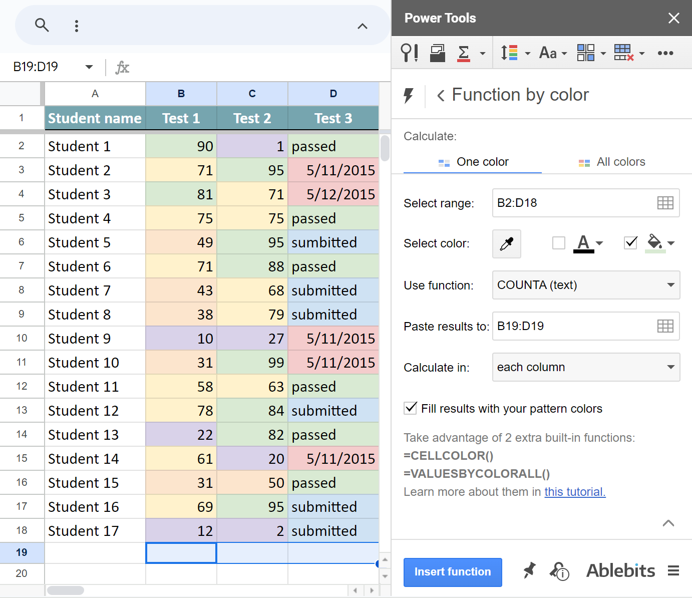
Here are six simple settings you need to specify to get the results:
- The range with the color-coded data that you want to check: I pick the columns with the test results, B2:D18.
- The pattern cell. The function will take its font and/or background color and look for the same in other cells. I pick the fill color of B2 as an example.
- The function. To count cells with a particular number format, it's best to choose the COUNTA function because it is the only one that works with non-numeric values. This way you can be sure that the data format in the cells will not impede the results.
- The place for results. I want my Google Sheets count cells by color in each column so it is three cells for me, B19:D19.
- How to apply it. You can choose to count cells in each row, column, or in all selected cells. As I want to count green cells for each test, I choose to Calculate in each column. If I wanted a general result for all three tests, I'd choose the entire range.
- The formatting of cells with the result. You can have them filled with the same colors as you count by selecting just one checkbox.
Once I click Insert function, the tool adds the formula under each column, so I will see the results for each test:
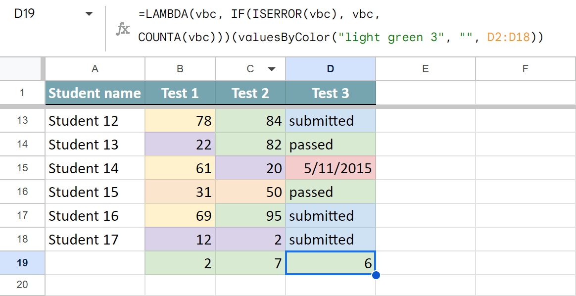
Let me break down its syntax and explain each part:
- =LAMBDA(vbc, IF(ISERROR(vbc), vbc is the service part that enables the formula to return exactly what Google Sheets replies with, whether it's "loading", some error, or the calculation result.
Tip. You'll see this part only for COUNT, COUNTA, and COUNTBLANKS functions because of their peculiarities.
- COUNTA(vbc) is one of standard Google Sheets functions you pick to use with the colored cells. vbc stands for valuesByColor.
- valuesByColor is our custom function that handles colors.
- light green 3 is the cell color considered for the calculations, i.e. the background color of the pattern cell.
- "" is empty since I don't consider the font color of the pattern cell.
- D2:D18 is the range to check for colored cells. In my example, it looks at cells in column B, C & D respectively.
How to sum colored cells in Google Sheets
Say, I'm keeping track of classroom equipment orders. I denote the ordered things by yellow background color, items on the way by blue, and delivered equipment by green:
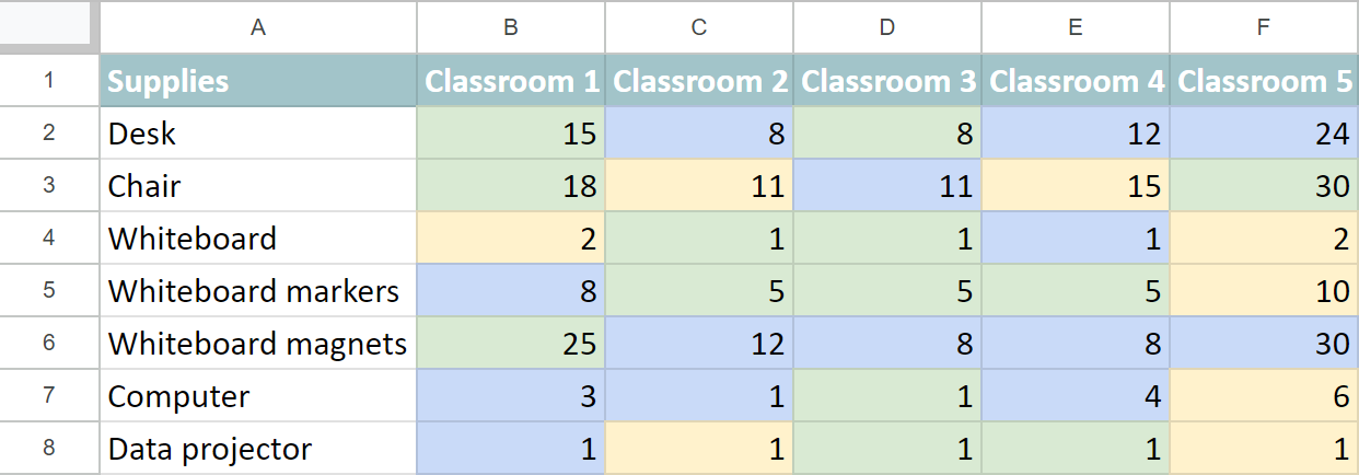
My task is to see how many desks, computers, and other supplies are on the way at the moment. Color is the only difference these numbers have in my table. So I open the tool to sum by color and use the following settings:
- I select the entire range with my data to check it, B2:F8
- I pick C2 as a pattern cell to specify the format of items I want to calculate.
- Select the SUM function to tally numbers from blue cells.
- Pick cells to place the resulting calculations for each item, G2:G8
- To see the number of shipped items for every product, apply the function to each row.
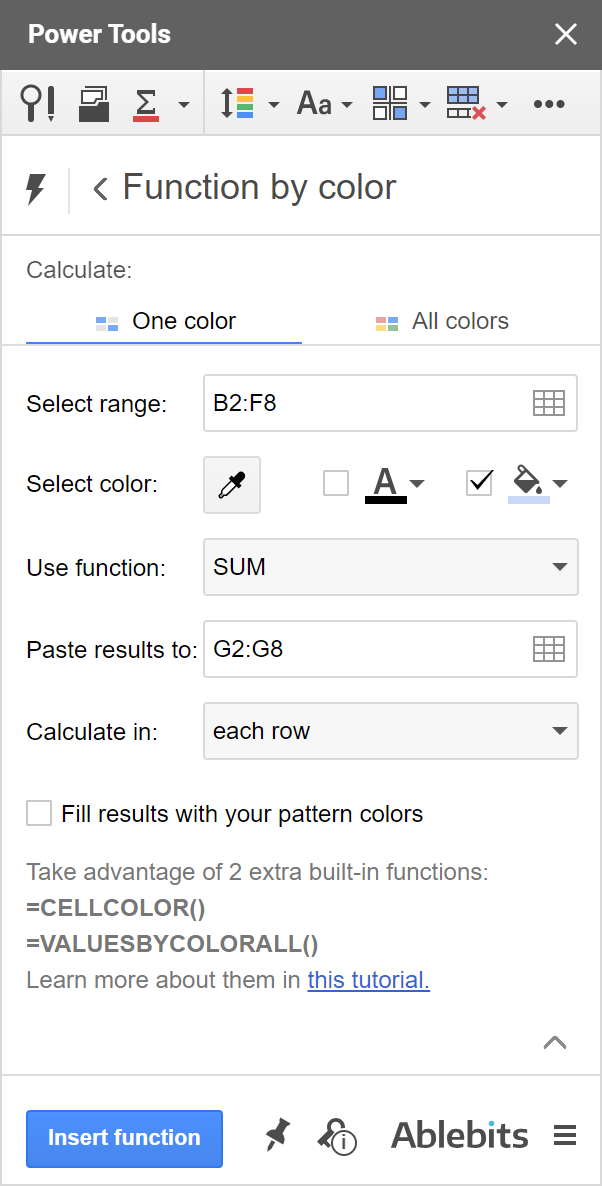
Click Insert function to get the formula after each line in your table.
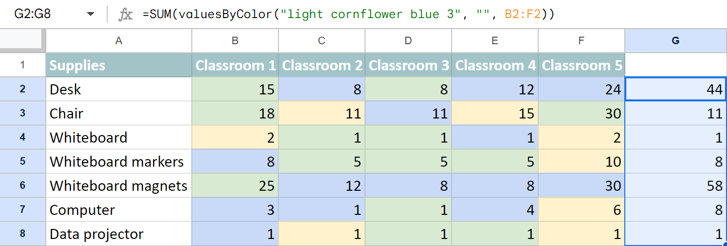
The convenience of getting the formula is that you can modify any of its parts and paste it wherever you need in your Google spreadsheets.
Google Sheets: sum by all colors in the table
The updated Function by Color lets you calculate not just one color per formula but all colors simultaneously.
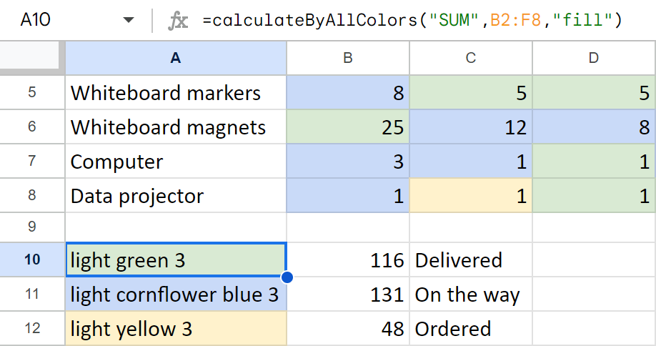
Using the same data as above, I can find the total of all delivered supplies (green), tally those on their way (blue) or those ready for ordering (yellow).
I just need to switch to the All colors tab in the add-on and adjust the same settings:
- The range is the same table, B2:F8.
- I will sum data by all fill colors.
- I also choose to calculate the entire range and have 1 formula inserted in A10.
Note. The formula returns the result in 2 columns: color & the total. So make sure there's enough space to insert the function. The result will show once there's room for it, but until then you may see the #REF! error if other data is on the way.
Update the results
So, Google Sheets doesn't have native functions that work with color. This means your spreadsheet doesn't treat changes to cell formatting as a reason to re-calculate your formula results. The good news is that both workarounds in-store are elementary :)
- You can change any value within the calculated range. Say, you are counting green cells in A1:C254. You can simply add a character to any of the cells in this range, and then remove it to get the updated results.
- If you have a lot of valuesByColor formulas in your sheet, click on the Refresh results option (right under the Function by color in Power Tools or under the Extensions menu for the single add-on) to update all formulas in one go.
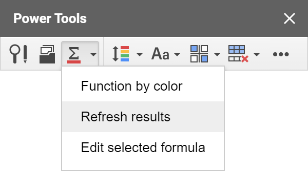
Edit formulas
Another way to change the result is to edit the entire formula. But if there are only a couple of settings you'd like to choose, you don't have to build the entire formula anew. It is enough to click a cell that already contains a formula and pick the option to edit it:
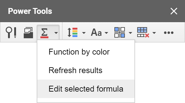
The add-on will open with all the settings necessary to create this selected custom formula. You can adjust some or all of them — ranges, colors, pattern cell, function — and insert everything back.
Troubleshooting
If you see an error in place of the formula, you may be working with a file that has no locale. When this happens, our function doesn't know what delimiters it should use, so it ends up giving you an error. If you see this, please go to File > Settings in Google Sheets and make sure you have the locale set.
Video: How to count colored cells in Google Sheets
 by
by
164 comments
Hi Irina,
I'm using the valueByColor function to count the number of cells in a range with certain background color, as exposed in this article:
=(COUNTIF(valuesByColor("#ffff00","",B7:AF7),""))
The above works as expected, detecting the cells in the range with yellow background. Nonetheless, when I do the same for the green background, it doesn't work at all:
=(COUNTIF(valuesByColor("#00ff00","",B7:AF7),""))
I can provide access to the google sheet so you can investigate this issue.
Thank you.
Hector:
There are many colors people call green and each variant has an individual hex code.
Here are some codes I found on the web by searching "color codes". Try some of these codes in your formula and see if one of them works.
lawngreen #7CFC00 rgb(124,252,0)
chartreuse #7FFF00 rgb(127,255,0)
limegreen #32CD32 rgb(50,205,50)
lime #00FF00 rgb(0.255.0)
forestgreen #228B22 rgb(34,139,34)
green #008000 rgb(0,128,0)
darkgreen #006400 rgb(0,100,0)
greenyellow #ADFF2F rgb(173,255,47)
yellowgreen #9ACD32 rgb(154,205,50)
springgreen #00FF7F rgb(0,255,127)
mediumspringgreen #00FA9A rgb(0,250,154)
lightgreen #90EE90 rgb(144,238,144)
palegreen #98FB98 rgb(152,251,152)
darkseagreen #8FBC8F rgb(143,188,143)
mediumseagreen #3CB371 rgb(60,179,113)
lightseagreen #20B2AA rgb(32,178,170)
seagreen #2E8B57 rgb(46,139,87)
olive #808000 rgb(128,128,0)
darkolivegreen #556B2F rgb(85,107,47)
olivedrab #6B8E23 rgb(107,142,35)
Hi, Hector,
If it's not a big trouble for you, yes, please share your spreadsheet with us (gapps.ablebits@gmail.com) with a description of your task.
We'll take a look at the problem and do our best to help.
La fórmula es: =SUM(valuesByColor("#00ff00"; "#000000"; Grupos!B4:B87))
Hi, Irina
I am troubled to figure out how to change a =sum formula based on the cell background color.
I have applied a color (black) conditional formatting to a column based on a text value (Canceled). Then I have color-matched another column with the "onEdit" function of the script editor based on the results on the first column, but I want the =sum formula on the second column which cells background color is black to automatically change to a zero value.
Is this possible to achieve? Thank you in advance for your help.
I have tried using your sum by color formula as instructed but keep receiving an error I don't understand:
"TypeError: Не удается прочитать свойство "sBackgroundPatternArg" объекта null. (line 3073)."
Hello Sandra,
Please go to File - Spreadsheet settings and set a locale for your file. This should fix the issue. Please let me know if it doesn't.
Hi! I have a sheet that I'm working with that I can't seem to get the Power Tool to refresh. I am trying to count a certain color in a range of cells. This is the formula I'm using:
=COUNTA(valuesByColor("#ffff00", "#000000", '1st Nine Weeks'!E5:I80))
I am only getting a response of 1 and when I go to refresh the arrows just keep twirling and nothing changes. Help please :) Thank you!
Hi Emily!
Sorry to hear that. Please make sure you have a locale selected for this spreadsheet (go to File - Spreadsheet settings). If it is set, could you specify if you are the owner of the document? Please also check what errors you see on the Console tab if you press F12 on your keyboard (Cmd+Alt+j if you have a Mac). We'll do our best to assist you.
I have cells that are color coded with dates in them. I want to get a count of cells that are a certain color and within the month of November. (eg (valuesByColor("#9fc5e8", "#000000", Sheet1!D3:D49), >=11/1/2017 and <=11/30/2017) I've been unable to get this to work. Can you provide the formula for this? Thanks.
Hi David,
Our function can't look at more than one condition. You can do this only with the help of an array formula, here is the one you need to use:
=sum(ARRAYFORMULA(--(11=arrayformula(month(valuesByColor("#9fc5e8", "#000000", Sheet1!D3:D49))))))
We hope this helps!
That works, thanks!!
Irina, sometimes this formula returns a 1 when it should return a 0. How can I fix that?
Hi David,
Could you share a sample spreadsheet with gapps.ablebits@gmail.com so that we can see what may be going wrong?
Hi there,
I'm using =COUNTA(valuesByColor("#6d9eeb"; 'Top Slice Full Scope'!D2:D59)) but it only counts 1 cell. If I use =valuesByColor("#6d9eeb"; 'Top Slice Full Scope'!D2:D59) it shows an error: Error
TypeError: Не удается прочитать свойство "sBackgroundPatternArg" объекта null. (line 3073).
Can you help?
Hi Marta,
Most likely the locale is not set in your spreadsheet and the function doesn't know what delimiter it should use. Please go to File - Spreadsheet settings and select some locale there, it should fix the issue.
I wish to count the number of cells with a particular value AND color.
How?
Jon
Hello Jon,
You can use the COUNTIF function for that, e.g.:
=COUNTIF(valuesByColor("#ff0000", "#000000", 'Sheet name'!A1:B100),"value")
Hi Irina - I have downloaded the add in as I want to sum by colour (I cam across your article on how to do this)
...However , the Sum by colour option is not showing in the formula dro pdown for sum
Can you advise ?
Thanks
Jim
Ignore that... User error!
I was looking in the auto sum drop down
Is there a reason why the tool won't count something that is in comparison? For example, I am trying to keep track of 2 different records like "3-1"... my current formula I have is...
=COUNTA(valuesByColor("#97f3c3","", G4:G11))&"-"&COUNTA(valuesByColor ("#ff9b9b","", G4:G11))
I have updated the spreadsheet settings > locale.
It is stuck at 1-1 for some reason.
Thanks in advance!
Hello Oscar,
I'm afraid one SumByColor formula can only calculate one color within one range. Please try to enter one formula for each color you want to count, and then subtract one result from another.
Ирина, большое Вам спасибо!
Очень долго боролся с проблемой по посчету ячеек по цвету.
И вам большое спасибо за отзыв, Станислав! Приятно слышать, что наше решение приносит пользу.
I am trying to count colored cells based on criteria in another column.
For instance, if column E2:E322 contains the text, "Wind ensemble," count the colored cell in the adjacent row F. I have a total count of colored cells in the row "F", but would like to split that by another criteria in another row.
I've also tried filtering the data into another spreadsheet, but the formatting doesn't copy using the filter tool.
Hello Chris,
I'm afraid Sum by Color doesn't support two conditions. You can try one workaround:
- Create one helper column for each color you want to check next to your data. Use Sum By Color with the "COUNTA" function and calculate "in each row". This way you will get "1" whenever the cell in column F has the color you are looking for. I.e. you should get the following type of formula in G2:
=COUNTA(valuesByColor("#9fc5e8", "#000000", 'Main sheet'!F2))
- Enter SUMIF function in another cell to count all cells with this color using the values in column G, while checking the necessary text value in column E as well:
=SUMIF(E2:E322,"Wind ensemble",G2:G322)
I hope this helps.
I am having trouble getting the Sum by Color to work. I have looked through all the comments in this thread, and not certain what I am doing wrong. I installed Power Tools, did the Sum By Color, selected the Pattern Cell Color, Source Range is from J15:J169, COUNTA, each column, results to E180. No matter which color I choose, the amount calculated is always 1.
Hi Becky,
Could you check if you have the locale set under File - Spreadsheet settings? If it is selected, would it be possible for you to share a sample spreadsheet with gapps.ablebits@gmail.com? We'll look into it.
Hi,
I want to only count the cells that have a fill of white (#ffffff) that have text in it?
Currently when i use the below formula it is counting the blank cells as well the cells that have text in it.
=COUNTA(valuesByColor("##ffffff", "#000000", 'Drawing Register'!A4:K706))
Can you provide some help on this?
Hi Zane,
As the COUNTA function includes blanks, you need your formula to calculate the difference between all cells formatted this way and empty cells:
=COUNTA(valuesByColor("#ffffff", "#000000", 'Drawing Register'!A4:K706))-COUNTBLANK(valuesByColor("#ffffff", "#000000", 'Drawing Register'!A4:K706))
Hi Irina,
thanks a lot for the add-on and all this useful comments. For this particular case the "COUNTA - COUNTBLANK" didn't work very well in the same function, returning 1 upon refresh. To whom may read for me the workaround was: "COUNTA" in a cell "COUNTBLANK" in another and then the simple difference "ex:a14-b14" in a third cell.
cheers :3
Thank you for your comment, Rob,
You are absolutely right, the current version of Sum By Color can't process more than one function at a time, sorry for misleading you. Good to know you found the workaround!
Good morning!
Thanks so much for the awesome add-on. When I try the Sum Color function, I keep getting an error that says "circular dependency detected". To my knowledge I do not have any other formulas in the sheet, so I am a little confused. Any help would be appreciated! Thanks in advance!
Hello,
Thank you for your feedback! Most likely you have the formula in a cell within the range you are trying to check. Please try to move the formula beyond the calculated range, it should work.
If you still see the error, please share a sample spreadsheet with gapps.ablebits@gmail.com, we'll look into it.
Hi, Irina!
First of all, thank you guys for this formula and for Power Tools! It's been working wonders around here!
However, I would like to combine this formula with a VLOOKUP. For example: I have a list of names and different values along multiple rows in another sheet and I have changed the BG color for some of these values. Something like:
Felipe 1 2 3
Irina 4 5 6
Felipe 7 8 9
I would like to know how many colored cells one name has. I tried using Sum By Color in an IF formula with VLOOKUP as its condition, but it didn't work.
=IF("Lance"=VLOOKUP("Lance";WEST!$B$2:$B$450;1;0);SUM(valuesByColor("#ff0000"; "#000000"; WEST!$C$2:$U$450)))
Is there a way I can make it work? If not, thanks anyway. The Sum by Color's been very helpful. 8)
Hi Felipe,
We really appreciate your kind words!
You're right, there is no straightforward way to count values by color and another condition as our tool doesn't support functions that work with more than one range. There is one workaround you can use if your sample values are in the same sheet:
- Add a helper column where you'll sum values by the necessary color in every row. E.g. if your numbers are in columns B:D, you will have this simple formula in column E:
=SUM(valuesByColor("#d9ead3", "#000000", Sheet18!B1:D1))
- Then sum values in column E by the necessary name in column A, e.g.:
=SUMIF(A1:A3,"Felipe",E1:E3)
Here is a link to your simple example:
https://goo.gl/jssi6z
If your task is different, please share a sample spreadsheet, we'll do our best to help.
Thanks, Irina!
I really tried to think of a workaround like you said, but couldn't come up with anything. Yours is a great idea, though. Thank you for that! I think it's gonna work!
Happy to hear it helps!
Hi, I find this tool very useful, but unfortunately, I could not get it to work. I tried updating my spreadsheet setting, but I end up getting a 1 as a result (I manually counted and it should be 285) here is the formula that I get from Google Sheet:
=COUNTA(valuesByColor("#f4c7c3", "#000000", 'Master File'!AF1:AF2110))
The source range though is in another sheet within the workbook. Your help will be highly appreciated.
Hi Rony,
Thank you very much for you feedback. Please check if you have the locale set in Spreadsheet settings under the File menu. If you do, please try to click on the Refresh option in Power Tools, and specify if you are the owner of the sheet and if it is shared with many people? We'll do our best to assist you.
Hi Irina,
Thanks for the speedy reply. Unfortunately, the "Refresh" option looks like it is cross out. I will share the work sheet with you via the gmail account. Though to answer some of your questions:
1. I am the owner of the Google sheet
2. It is shared with 3 other people.
I will request the other 3 to update their setting also, as that might be the issue.
Again thanks for the speedy response.
Regards,
Rony
Hi Rony,
Please share the spreadsheet with gapps.ablebits@gmail.com
Please also send us a screenshot of the Refresh option the way you see it, we'll look into it.
Thank you for your time.
I'm either getting lostin directions or what I want isn't possible. I'm trying to calculate how many time a red colored cell appears in a row. Is there any way you can simplify this?
Hi Morgan,
Here are the steps you can follow to do this:
- Start Power Tools, click on the little arrow next to AutoSum tool at the top and select the Sum by Color tool to open it
- Pick any red cell as your pattern cell
- Select the range with all your data for the "Source range"
- Select the "COUNTA" function
- Choose the option to calculate in each row
- Select the top cell for the calculation results in the last field
- Click "Insert function"
If you still have any issues, please share a sample spreadsheet with gapps.ablebits@gmail.com, we'll look into it.
IP, I have the need to count the # of rows, in a 3 column span, but wasn't able to figure out how to get the range of columns figured out from the examples. I Used the following function and it appears to be working great on a single column (K).
=COUNTA(valuesByColor("#f4cccc", "#000000", 'Review Compare'!K5:K567))
Any thoughts on how I would count the total # of rows that have a specific bgcolor for columns I, J & K?
Thanks, KB3
Hello KB3,
I'm sorry, but our function can only count the number of cells by color, it can't calculate the number of rows.
Hi
I keep receiving the error "Range Not Found", not sure what is going on here? Any advice?
Hi Stephanie,
Thank you for contacting us. Could you specify if you select the range in the same spreadsheet when you insert the function?
Please send a screenshot of Sum By Color settings you choose and of the formula you get as a result to gapps.ablebits@gmail.com.
We'll look into this issue.
Hi Irina,
Thank you I will send you a screen shot. The range I am using is the range of 1 column with multiple cell colors//values. I would like to get the sum of each cell color.
Hi Stephanie,
Thank you for the screenshot.
The locale was not set for the file and the function couldn't calculate the results without knowing the delimiter it should use. If this happens again, please go to File -> Spreadsheet Settings and make sure Locale is selected, then start Power Tools and refresh the results.
Feel free to contact me again if you have any other questions.
Hi there,
Is it possible for the formula to count data from multiple sheets? ie: Q1!A6:CM6, Q2!A6:CM6, etc?
Thanks!
Marielle
Hi Marielle,
Though it is not possible in one formula, you can create a master formula for the results of Sum By Color from each sheet, e.g. if you have the results in cell A7 in Q1 and Q2, you can enter the following formula into A8 in Q1:
=A7+Q2!A7
hi -- thanks for this article – it's exactly what i'm looking for. I keep getting this error in the cell:
Error
Circular dependency detected.
Do you know what I might be doing wrong?
thanks,
james
Hi James,
You must have inserted the formula into the range where you are trying to count cells by color. Please enter it in a cell outside of the calculated range, this should fix the issue.
Please let me know if you have any other questions.
Hi Irina,
When I do the =sum(ValuesByColor), all my inputs are fine and I'm able to follow all the steps. However my results end with an #ERROR! – either "Formula parse error" or "TypeError: Не удается прочитать свойство "sBackgroundPatternArg" объекта null. (line 3047)."
What am I doing wrong, and how can I fix this?
Thanks
Hi Esther,
Please go to File - Spreadsheet settings and select a locale there, this should fix the error.
Please let me know if it doesn't.
Hi Irina,
What I want is to give me an exact number of cells shaded in red - these cells does not have value/data in it, just purely shaded. How to go about his please.
Hi Lea,
As long as the range you are checking is not completely empty, i.e. at east one cell has some data in it, you can select COUNTA function to get a number of all cells with a particular color.
I just realized that I could not get results unless I added all colored cells before adding formula. Actually, I would like to add the formula first, then as people add colors in certain cells calculation occurs. Do you have any devices for those needs? Thank you.
Hello Ling,
You can still use Sum By Color, but you will need to click "Refresh" to see the results. Functions in Google Sheets do not update formula calculations when the background color changes. We can't affect this behaviour, which is why we introduced the "Refresh" option, you can find it right under Sum By Color. You can also change just one of the values in the calculated range instead, e.g. add and remove a character, the results should be updated then.
It appears that when you chain calls to valuesByColor within the same formula the result is computed incorrectly. For instance:
=COUNTA(valuesByColor("#f4cccc", "#263238", '2016'!J33:X37))
Returns :: 17
=COUNTA(valuesByColor("#f4cccc", "#263238", '2016'!J33:X37))+COUNTA(valuesByColor("#f4cccc", "#263238", '2016'!J33:X37))
Returns :: 68 (oddly 17+17+17+17)
Or as another example
=COUNTA(valuesByColor("#f4cccc", "#263238", '2016'!J33:X37))
Returns :: 17
=COUNTA(valuesByColor("#f4cccc", "#263238", '2016'!J33:X37))+COUNTA(valuesByColor("#f4cccc", "#263238", '2016'!B42))
Returns :: 36 (which we will note is 17+1+17+1)
Of course a valuesByColor of a single cell can return only a 0 or 1
Is there something about the operation of the function that I am missing?
Hello,
You are right, the function can't process more than one color in one formula, you need to enter a formula for each color you want to count. To combine the results, add a master formula that will sum them up, i.e. if you have the results by color in cells J38 and J39, then enter =SUM(J38, J39) in a different cell.
We will consider adding the possibility to process more than one color in one of the future versions of the add-on.
Please let me know if you have any other questions.
In all cases provided the functions are only processing one color over multiple calls. I gather though that you response means that multiple calls to the valuesByColor function within the same formula contaminate the result due to compounding each call into the following.
Thanks.
Sorry for misinforming you. The issue is not only with the color, but with different ranges within one formula. When Google Sheets launches a custom function, we don't have the technical possibility to know which of the functions from the formula it processes when there are 2 or more of them. We always read the first range, which is why using the same ValuesByColor function in one formula is not possible. Our developers are looking for ways around this issue.
Hello,
We have been enjoying this function for a while with no problems. It is used on Google Form responses sheet where conditioning formatting is added. For some reason all results are showing 1. Tried refreshing but loading seems to happen in the other columns. It works just fine on brand new sheet.
What might be the issue?
Hello Jurate,
Thank you for your feedback. Please check if the locale is selected in File -> Spreadsheet settings. If it is, could you share the spreadsheet with gapps.ablebits@gmail.com? We'll look for the reason why the function may not work there.
Hey Irina,
Thanks for this detailed & thorough breakdown - it will work for me eventually I'm sure but at the moment it's not, and I'm sure you can help me crack it!
I've got a column filled with either Yes or No, with each cell possessing the conditional formatting of 'If text contains 'Yes' the cell turns green' and 'If text contains 'No' the cell turns Red'.
I've tried following the steps, trying to add up the total of Yes-Green cells I have in the column, and it keeps returning a value of '1' when there's clearly more than 1 cell labelled Yes.
Any ideas or help you can offer?
Thanks a bunch!!!
Michael
Hi Michael,
It looks like some error occurs when trying to calculate the results.
First please make sure you use the COUNTA function as it is the only one that works with text values. Please also check if you have a locale set in "File-Spreadsheet settings".
If this doesn't help, would it be possible for you to share a sample spreadsheet with gapps.ablebits@gmail.com? We'll do our best to assist you.
Hi -
Great add-on! As always, with solutions come further questions!:
Is there a way to use this formula [valuesByColour] as a criteria within another formula?
i.e. Of those cells formatted in RED, how many contain "XYZ" ?
I am trying to build a formula using COUNTIFS, in this way but am having no luck. Is there a better way to do this, or can this not be used as a criteria?
Hello Lucy,
Thank you very much for your feedback!
You can use our custom function as a criterion within another formula, e.g.
=COUNTIF(valuesByColor("#ff0000", "#000000", Sheet1!A1:E12),"xyz")
If this doesn't help, could you please describe your task in more detail?
Hi Irina,
That's perfect. Thank you!
I think I was trying to add too many components!
Thank you for the update, Lucy!
Feel free to contact me if you have further questions
Hello,
The powertools are working great for me. My problem is I would like to have it Count two colors.
Like =COUNTA(valuesByColor("#00ff00" ; "#ff0000"; ""; Ark1!D2:D11))
Which should count green and red background colors? or I would like it to do that.
Hello Troels,
We haven't provided for a way to process more than one color at a time, so you need to enter one formula for each color you want to count. The only way to combine the results now is to have a master formula that will sum up the results by each color, i.e. if you have results by color in cells D12 and E12, then enter =SUM(D12, E12) in a different cell to get the result you need.
We will consider embedding this possibility in one of the future versions of the add-on.
Please let me know if you have any other questions.
P.S. In a row with no colored cells, it also puts a 1 when it fails.
Hello,
I'm sorry to hear that you are having difficulties with the add-on. Would it be possible for you to share a sample spreadsheet where this issue occurs with gapps.ablebits@gmail.com? If you have any sensitive data, you can replace it with irrelevant information, just keep the format. We'll do our best to find what is causing this issue.
I'm having the same problem mentioned above where when I run a refresh, it stays for some seconds and then goes back to 1. The weird thing is that I have about 80 rows and am using the count color function in two columns (with counta). When it fails, it fails in both columns, but it was working fine before I did some sorting. Now it's back to its pre-sort form, but about 7 scattered rows are having this problem. I did check the locale, and it says U.S. I've tried replacing them from Power Tools as well as by copying the cells above that are working. No go. Quite frustrating.
Hello,
I am using Sum by Color, but the number doesn't seem to update when I add or remove a color from the range it is counting.
I had 9 "moderate green" cells (#92d050) which it counted perfectly. When I went back later to add another moderate green cell in the range, it did not update to 10. The font color was the same on the newly added cell, also.
Any hints? Here is the formula being used:
=COUNTA(valuesByColor("#92d050", "#000000", Sheet1!C116:C150))
Silly me, didn't try the refresh on Power Tools.
But I do have a follow-up question. This is a shared doc with my colleagues. If they don't have pro, is there a way for them to refresh the values? It seems simply closing and reopening the Sheet does not resolve that problem.
Hello Meghan,
You see, functions in Google Sheets do not "see" background color modifications, they update the results only when the values change. There is nothing we can do to resolve this, which is why we added the option that refreshes SumByColor results.
If your colleagues do not have Power Tools, they can change just one of the values in the calculated range to trigger an update, for example add and remove a character.
The tool does not seem to like negative numbers. Trying to add up numbers exported from a bank statement and it returns zero when it encounters a negative number.
Hello Evelyn,
I'm sorry, but we couldn't reproduce this issue. Could you please specify what function you select for the formula? If possible, please share a sample sheet where this occurs with gapps.ablebits@gmail.com, we'll look into it. If you have any sensitive information, you can replace it with dummy records, just keep the format.
I am having zero success. I am trying to add a column of values that are color coded. I only want to add specific colors into different fields. The Sum by Color option on the Power tools and the instructions are not working. This is the formula it gives me =SUM(valuesByColor("#d99594", "#000000", '4 Week Cycle'!N3:N6))
Could you please specify what you see as the calculation results? Please also make sure you have a locale set in File - Spreadsheet settings.
I want to to use cells like a gantt chart with 1 cell = 30min.
Is there a way assign a value to a cell in such a way or can it only count a coloured cell as a 1?
Hello Joel,
If you want to take each colored cell as 30 minutes and get the result in hours : minutes, just divide the formula result by 48 (e.g =COUNTA(valuesByColor("#b6d7a8","", B2:B40))/48 ) and apply the Time format to the cell.
Hi,
When using sum by color and counting the number of cells that are a particular color. If there are no cells of that color, I don't want it to return a "0". Just a blank cell. Is there a way to do that?
Rick
Hi Rick,
There are two ways you can do this:
1) You can use an IF statement, e.g.:
=IF(COUNTA(valuesByColor("#f4f4f4", "#000000", B8:F11)),COUNTA(valuesByColor("#f4f4f4", "#000000", B8:F11)),"")
2) You can use Conditional formatting in Google Sheets and choose white font color for zero values to hide them
I'm trying to use this tool in a sheet but when I run the count by color formula, it shows the result of 1. There should be 2 or more for any given color. Any ideas?
Sample sheet: https://docs.google.com/spreadsheets/d/10x5Tm4XZCrYqUd6EzXwVRiDRjExrvRP70uEvzKUryR4/edit?usp=sharing
Hello Sarah,
Thank you for sharing your sample spreadsheet. Could you please make sure the locale is selected for your spreadsheet under File – Spreadsheet settings?
If it is, please let me know if you inserted the function using the add-on, or entered it manually? We can’t seem to reproduce this issue, here is an example of the spreadsheet I created with the same data, you can see that the function calculates the results correctly:
https://docs.google.com/spreadsheets/d/18v73MeMKfjBYYHbxwtRVAorDQLYehObfNMOMeBWE-bU/edit?usp=sharing
Wow, you are very responsive to your users! I wanted to count by color but, unfortunately, my company does not allow add-ins for google sheets.
Thank you very much for your feedback, Greg! I'm sorry that you can't use add-ons. If you happen to work with Microsoft Excel as well, you can try our on-premises add-in for this task:
https://www.ablebits.com/excel-count-sum-color/index.php
Hi, this is working great. How would I filter the sheet that it will only count the colours of the cells if it matches a date greater than something I will specify ?
Any tips ?
Hi Andri,
There are two ways you can do this. As our function can check only the color of the cells, you can combine it with the COUNTIF function in Google Sheets, e.g.:
=COUNTIF(valuesByColor("#b7e1cd", "#000000", Sheet11!I2:I38),">="&I3)
Here I3 is the date to compare against.
You can also use conditional formatting first:
- Go to Format -> Conditional formatting, choose to format cells if date is after exact date, enter your criterion and click Done;
- Run Sum by color to count the formatted cells
Hello there.
Been trying multiple add ons on Google sheets. to count the sum of values in a particular colour.
Finally, I am really close.. Thanks to your add on.
My only other need is,
The Power Tools gives me only 3 options
"Insert function after: Entire range, Each Column, Each Row"
Would it possible if I can insert / call the function in a cell on another page of the same excel sheet?
Appreciate your help in advance :)
Justin
Hello Justin,
Thank you for your question.
We are actually about to publish a new version of the add-on that will let you choose where to paste the results. You will still be able to add calculations for the entire range, each row, or each column.
Now you can copy the formula to any place in the spreadsheet. However, if you want it to look at a different sheet, you need to include its name into the range like you do in regular formulas, e.g.:
=COUNTA(valuesByColor("#d9ead3", "#000000", 'Sheet1'!D1:H11))
Please let me know if you have any other questions.
This is great, thank you. I did it and it was working perfectly fine yesterday. However, when I came back today to the sheet I had set it up on, the values are stuck on "Loading" and when I click on the cells it is telling me that 'valuesbycolor' is an unknown function. Opening up power tools and hitting refresh is not helping. Do I really have to go through the process of setting up the valuesbycolor every single time I use it?
Hello Em,
I'm sorry to hear that you are having difficulties of this kind. It sounds like this is related to an issue with custom functions in Google Sheets that hasn't been resolved yet:
https://code.google.com/p/google-apps-script-issues/issues/detail?id=4156
However, please share a sample spreadsheet where it is reproduced with gapps.ablebits@gmail.com if possible, our developer will look into possible reasons why this may be happening.
Mine only counts purple cells with text. I need ALL the purple cells... (campsites occupied, on my data sheet)
The only function that works with blank values is COUNTA, please use it in your ValuesByColor formula to get a count of purple cells.
Hi there,
I want to count my green cells and when i make the function with power tools it works.
But when i close the document and open again. If i add more green cells the counter does not change.
How can i fix it ?
Can i work with it in the mobile too ?
Hi André,
You see, functions in Google Sheets do not consider the change of background color as a reason to update the results. We can't affect this behaviour, so we introduced the "Refresh" option for our Sum By Color function. You can see it right under Sum By Color in the toolbar of the Power Tools add-on. As an alternative, you can change just one of the values in the calculated range, e.g. add and remove a character, to trigger an update.
Add-ons are not supported on the mobile platform.
I hope that you'll find this information helpful.
Hi
Does it still working as what I get currently if documents is share and view by collaborator who does not install power tools?
Hi Nulrek,
If you insert the function using Power Tools and then share this spreadsheet with other users, the function will work. When you go to Add-ons -> Manage add-ons, please make sure Power Tools has the "Use in this document" option selected.
There is one thing to keep in mind though: as custom formulas are not refreshed automatically, other users can update the results by changing any value in the range used in the formula, e.g. enter and remove a character.
Hi there!
When I use the formula =valuesByColor("#ff0000"; "#000000"; C9:L47) it returns the values that I'm looking for but when I use =count(valuesByColor("#ff0000"; "#000000"; C9:L47)) it just returns 0.
Any thoughts?
Thanks!
Nevermind, solved it using counta.
Thanks!
Thank you for the update, Cristóvão!
having the same problem. any suggestions on how to resolve this?
Hello,
If selecting "Refresh" from Power Tools doesn't resolve it, would it be possible for you to share the spreadsheet where this issue occurs with gapps.ablebits@gmail.com? We'll look into it.
Hi Irina
I have installed the Power Tools Add-on and would to use the Sum by Color funtion. For some reason it doesn't show me the Insert Function button as in your example. Am I missing something here?
Many thanks!
Hi Eugene,
Thank you for contacting us.
Could you please make sure that your browser page is not zoomed in? Please try to press Ctrl+0 (or cmd+0 if you have a Mac) or make sure you have 100% in the browser settings -> Zoom.
If this doesn't help, please go to Control Panel\Appearance and Personalization\Display and check what sizing option you have set there.
Please let me know about the results.
Hi,
i have a table where cells are both empty and filled.
I want to count the blank cells in a specific background color.
I tried with Powertool Sum by color + countblank .. but it returns zero where i know it should return quite a high number instead.
Could you help?
Hi Mishelle,
I'm sorry, but we couldn't reproduce this issue. Please try to remove the standard function from the formula and see if you get any errors. E.g. if your formula looks the following way:
=COUNTBLANK(valuesByColor("#b6d7a8", "#000000", C1:D9))
Try to make it look like this:
=valuesByColor("#b6d7a8", "#000000", C1:D9)
If possible, please also share a sample spreadsheet where this issue occurs with gapps.ablebits@gmail.com
We'll look into it.
When I click refresh, the spinner goes on forever... My sheet has 15 counta by color cells only. What gives?
Hello Brandon,
Thank you for contacting us.
When you see this again, could you please press F12 on your keyboard (Cmd+alt+j if you have a Mac), go to the Console tab, and check what errors you see highlighted in red? Please send the text of the errors to us, our developer will look into this issue.
Hey Guys,
For some reason the code is working perfectly but after a short period of time it is showing 0 result for all count formula.
Reseting the sheet will display the correct counts again but only for a brief period, maybe 20 seconds.
Do you have any idea what might be causing this?
Hello Adam,
I'm sorry to hear that you are having difficulties with the add-on.
Could you please try to insert the same function from Power Tools and check if it behaves the same way?
If it does, try to remove the standard function from the formula, e.g. =valuesByColor(A1,A1,A1:B10)
Please let me know what error you see in the cell.
Hello Irina,
I am having same issue as Adam mentioned above although I did exactly step by step you guided in this page.
I tried many times and have same the result - it gives zero value for count/sum formula so I suppose this add-on is not perfect one to help us in counting/summing values by colored cell.
Thank to check it on your side and any advice from you to solve our issue are highly appreciated.
Hello Quang,
Would it be possible for you to share a sample spreadsheet where this issue occurs with gapps.ablebits@gmail.com? We'll look into it.
That is because the app is limited for one use per day unless you give them money.