The article shows how to consolidate multiple cells, sheets, and files in Excel and explains which method works best in different situations.
Many Excel users work with data scattered across several worksheets: one per month, per region, or per employee. If you've ever copied and pasted information from different sources to create a report, you know how time-consuming it can be. Excel's Consolidation can help by automatically combining values from multiple ranges, sheets, or files into one clear summary.
Note. The consolidation methods in this tutorial are meant for summarizing numeric data. If you are looking to merge worksheets by copying their content, refer to How to combine Excel spreadsheets into one.
What is data consolidation in Excel?
Data consolidation in Excel is a way to combine data from multiple sources into a single summary. These sources can include separate ranges, different sheets within the same workbook, or multiple files. Instead of reviewing each dataset individually, consolidation brings aggregated results such as totals, counts, averages, or other calculations into one place.
This approach is commonly used when you work with similar data, for example, monthly sales or regional reports, and want an overall summary.
It's important to note that consolidation does not copy source data into one place. Its purpose is to calculate and present summary values based on matching positions or labels, helping you see the bigger picture at a glance.
Excel lets you combine data in several ways. You can leverage the built-in Consolidation tool, apply formulas, or use pivot tables for more flexible summaries. The method you choose depends on how your data is organized and how often it changes.
How to consolidate data in Excel
A quick way to aggregate data from multiple ranges, worksheets, or workbooks is by using the built-in tool.
Here are the basic steps to consolidate in Excel:
- Prepare your data. For the Consolidate feature to work correctly, make sure that:
- Each range has the same layout and structure.
- Each column has a header and contains the same type of data.
- There are no blank rows or columns within the datasets.
- Select the destination. In the worksheet where you want the results to appear, click the upper-left cell of the output area. Make sure there is enough empty space to the right and below this cell so existing data is not overwritten.
- Run the Consolidate tool. On the Data tab, in the Data Tools group, click Consolidate.
- Choose a function. Select how Excel should summarize the data, such as Sum, Count, Average, Max, or Min.
- Add source ranges. Click in the Reference box and select the first range, then click Add.
To include ranges from another workbook, click Browse and locate the file. - Use labels (optional but recommended). If your datasets include headers, you can choose to use labels. This allows Excel to match data correctly by row or column headers rather than by position.
- Create links to source data (optional). To have the consolidated results update automatically when source data changes, select Create links to source data. In this case, Excel inserts formulas that reference the original ranges instead of producing a static summary. Keep in mind that links can't be created when the source and destination ranges are on the same worksheet.
- Create data summary. Click OK to finish the process. Excel will create a summary table based on your settings.
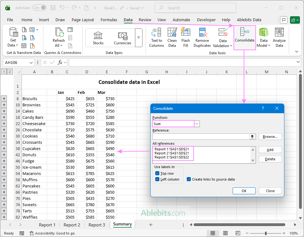
Best to be used for: Summarizing numeric data from multiple sources with similar layouts.
Two ways to consolidate data from multiple sources
Excel provides two main ways to consolidate data from multiple datasets. The method you choose depends on how your source data is arranged and whether labels are consistent across datasets.
Consolidate by position
This method can be used when all source ranges have the same layout, with data arranged in the same rows and columns. Excel combines values based on their cell positions, i.e. values that appear in the same location in each range.
In this case, you may or may not choose the Use labels options. However, if you do not use labels, the result will include only aggregated numeric values, without row or column headers.
This method works best when you are working with standardized reports, where:
- All worksheets follow the same structure
- Rows and columns appear in the same order
Consolidate by category
Consolidation by category is used when the source ranges are arranged differently but have the same row and column headers. Instead of relying on cell position, Excel combines values based on matching labels.
This method only works when you select one or both options under Use labels:
- Top row to match data by column headers
- Left column to match data by row labels
Without selecting these options, Excel has no way to identify which values belong together, and consolidation will not work correctly.
Now that you know the essentials of the Excel Consolidate feature, let's look at how it works in different scenarios. While the starting steps remain the same, the choice of summary function and data-matching method determine the final layout of the results.
How to consolidate cells in Excel
Let's start with a simple example using a single range. The source table contains multiple records for different departments, and the goal is to sum up values from multiple rows into one total per department.
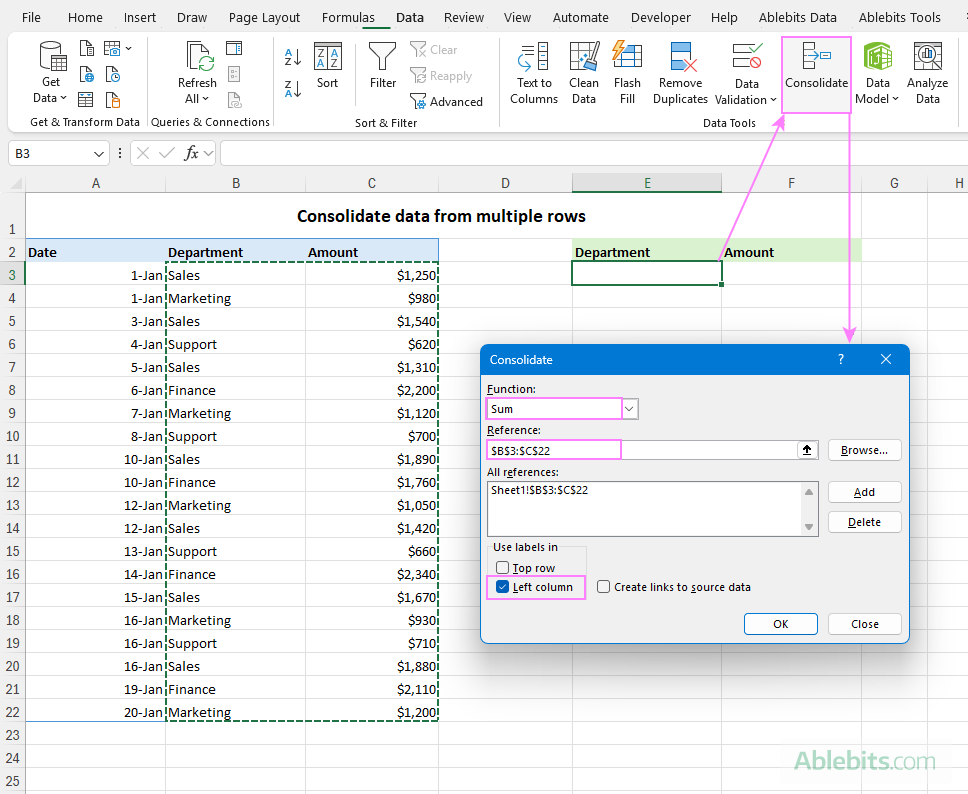
- Select the starting cell. Because the consolidation will take place on the same worksheet, select the cell where you want the results to appear (cell E2 in this example). Make sure there are enough empty columns to the right and rows below to hold the consolidated data.
- Open the Consolidate tool. Go to the Data tab > Consolidate.
- Choose the function. Select Sum to add up related values.
- Select the source data. Click in the Reference box, then select the data range with your mouse.
Click Add to include it in the All references list. - Use row labels to match the data. As we aim to summarize amounts from multiple rows, choose to use the labels in the Left column.
- Click OK to generate the results.
The result is a summary of the selected range, with totals calculated for each department.
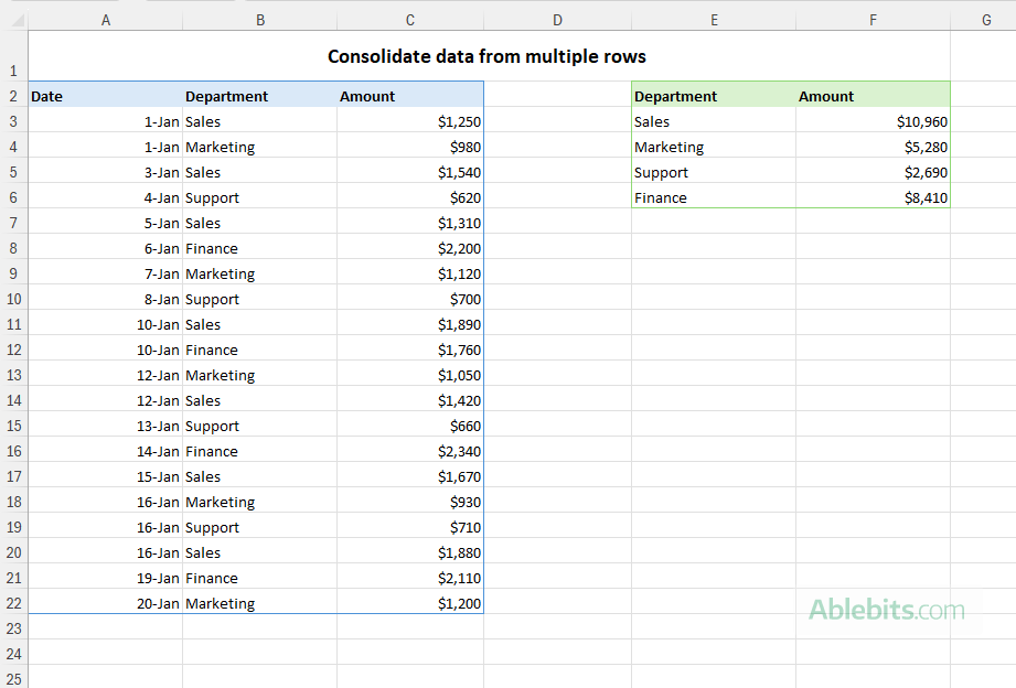
Note. Since the source data and the results are on the same worksheet, Excel can't create links to the original data. As a result, you'll need to run the consolidation every time the original data is updated. If you want the results to refresh automatically, consider using formulas or pivot tables instead.
How to consolidate sheets in Excel
Combining data from multiple worksheets is where Excel's Consolidate feature really proves its value. It enables you to gather info from different sheets and produce a single master report in just a few steps. Let's see how this works in practice.
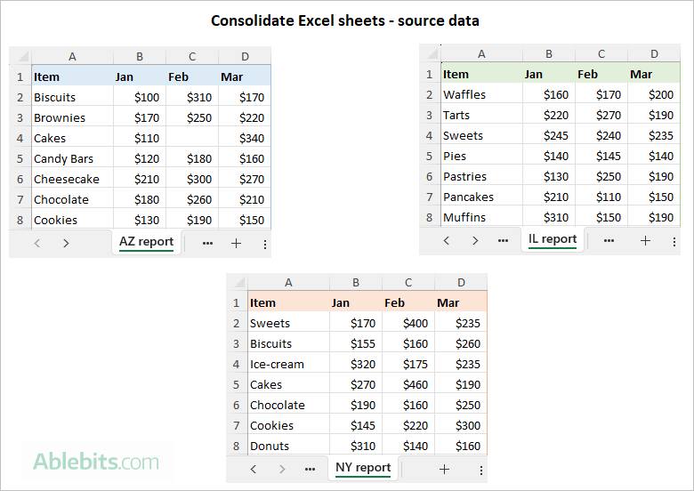
Suppose you receive sales reports from several regional offices, each stored on a separate sheet. Your goal is to combine those figures into one spreadsheet that shows total sales for each product.
Steps to consolidate data from multiple worksheets:
- Review the source data. Before you start, check that the worksheets you want to combine share a similar structure, consistent data types and column headers. Worksheets may have different numbers of rows and rows can be arranged in a different order, which is fine.
- Run Excel Consolidate. In the master worksheet, select the upper-left cell of the destination range. Then go to the Data tab > Consolidate.
Tip. It's best to consolidate data into an empty worksheet. If the master sheet already contains data, ensure there is enough blank space (rows and columns) to hold the summary.
- Configure the consolidation settings:
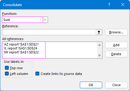
- Choose the summary function. Select how the data should be combined. In this example, we choose Sum.
- Add source ranges from different sheets. Click in the Reference box and select the range on the first worksheet, then click Add to include it in the All references list. Repeat this step for each worksheet you want to consolidate. You can also use the Collapse Dialog button to make selecting ranges easier.
- Choose how to match data. Under Use labels, select Top row, Left column, or both to match data by column and/or row headers.
- Choose how the results update. Select Create links to source data if you want the results to update automatically when the source data changes.
- Click OK to create the summary.
Consolidation result
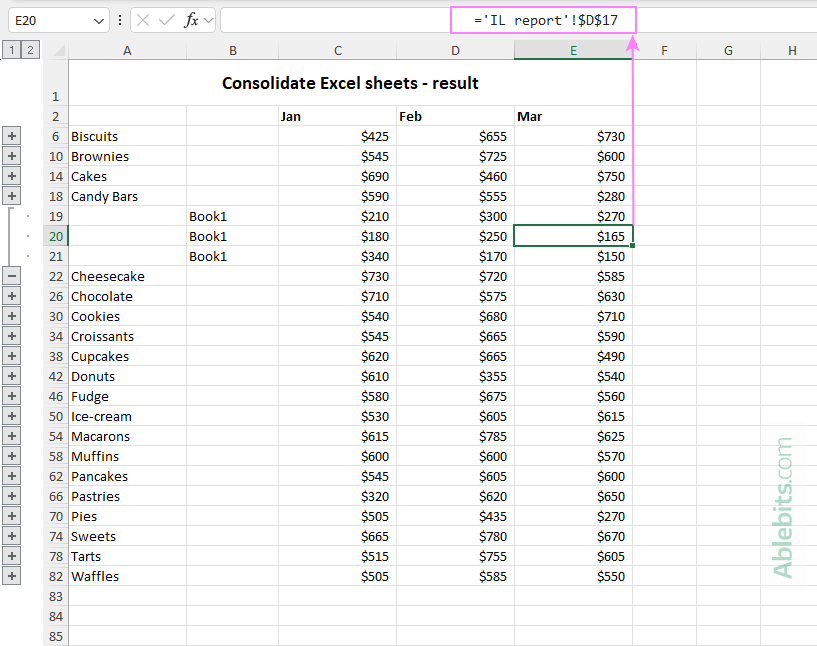
With the Create links to source data option selected, Excel produces an outlined summary similar to the one shown below. The results are formula-driven. You can confirm this by selecting any numeric cell in the output and checking the formula bar.
To see where a specific value comes from, expand an outline group by clicking the plus (+) icon. Then select a value, and Excel will show a link to the original source cell in the formula bar.
As you can see, the Consolidate tool is very helpful for aggregating numeric data from multiple worksheets. However, it's not the only way. A 3D reference can be a simple alternative to summarize data in consecutive sheets using a single formula.
How to consolidate Excel files into one
When your data is spread across multiple files, Excel's Consolidate feature can handle this as well, provided all source workbooks are structured consistently. The process is very similar to combining data from multiple worksheets, with the main difference being that the ranges come from different files.
Below is a brief outline of the steps:
- Open the destination workbook. Create a new workbook or open an existing one that will hold the consolidated results. Select an empty worksheet or ensure there is enough blank space for the summary output.
- Start the Consolidate tool. Select the upper-left cell of the destination range, then click Consolidate on the Data
- Set up consolidation:
- Choose a summary function. Choose the function for aggregating the data.
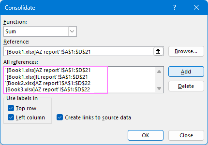
- Add ranges from different workbooks. Click in the Reference box and select the data range from the first workbook. Click Add to move it to the All references box.
Repeat this step for each sheet you want to include. Use the Browse button to locate files that are not currently open. - Match data using labels (recommended). Under Use labels, select the option to consolidate data by column and/or row labels rather than by position. This ensures that related values will be matched correctly, even if rows or columns appear in a different order across worksheets.
- Create links to source data (optional). Select Create links to source data if you want the results to update automatically when the source files change. Keep in mind that the source workbooks must remain accessible for the links to work.
- Click OK to create the summary.
Resulting summary
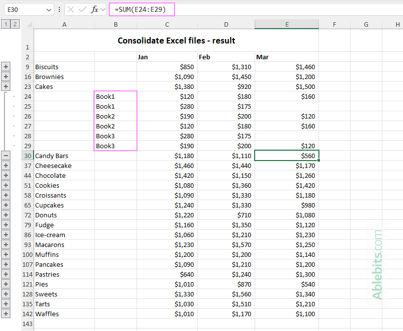
Excel combines values from all selected workbooks into a single summary. If links were created, you can expand the results to see which file each value originates from.
Tip. If you need to copy sheets from different workbooks, see How to merge multiple Excel files into one.
Consolidating data in Excel using formulas
Excel formulas offer a flexible way to combine data in cells, columns, or ranges. To summarize numeric values, you can use SUM, AVERAGE, MAX, and MIN or their conditional counterparts such as SUMIF.
If your worksheets have identical structures, you can also use:
- 3D references to summarize sheets in the same workbook.
- External references to aggregate data from different Excel files.
Formula results update automatically when source data changes, which makes them especially useful for ongoing reports or workbooks where data is frequently updated.
Best for: Simple calculations, identical worksheets, and cases where you want direct control over formulas.
How to consolidate rows in Excel
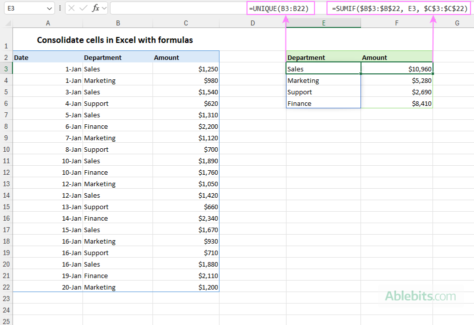
To consolidate numeric data from multiple rows in Excel, a simple formula is often all you need. As an example, let's see how you can quickly sum amounts by department in the dataset below.
First, apply the UNIQUE function to extract a list of department names from column B:
=UNIQUE(B3:B22)
Next, use SUMIF to add up values that belong to each department. More precisely, the formula sums up the values in column C for rows where the department in column B matches the name in cell E3.
=SUMIF($B$3:$B$22, E3, $C$3:$C$22)
The results are exactly the same as those produced by the Consolidate feature, but with one important difference: the totals update automatically whenever the source data changes.
In your own worksheets, you may need to use different formulas depending on how your data is structured.
How to consolidate columns in Excel
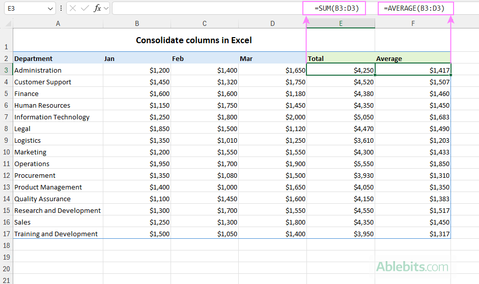
Consolidating numeric data from multiple columns can also be done with standard summary functions. This approach works especially well when related values are stored in adjacent columns and need to be combined row by row.
For example, to calculate the total of the numbers in columns B, C, and D for each row, enter the following formula in cell E3, then copy it down to the remaining rows:
=SUM(B3:D3)
To calculate an average instead of a total, apply the AVERAGE function in the same way:
=AVERAGE(B3:D3)
Consolidating text values from multiple columns
Sometimes, you may see the term consolidate applied to text values, although combine is a more accurate description in this case. Excel provides several functions for combining text from multiple columns into one cell:
- CONCAT – merges text values from multiple cells or ranges.
- CONCATENATE – combines text strings (older function, still supported).
- TEXTJOIN – joins text from multiple cells with a specified delimiter.
Other tools for consolidating data in Excel
Aside from the built-in Consolidate feature and formulas, there are a few other tools to bring data together in Excel. Depending on how your sheets are structured and how much control you want over the results, you can use one of the following options.
PivotTables
PivotTables let you summarize and group data dynamically without writing formulas and without changing the source data. They make it easy to calculate totals, counts, averages, and subtotals, and to rearrange the layout as your analysis evolves.
However, pivot tables work with a single dataset only. They cannot combine data from multiple sheets or workbooks. Before using a pivot table, all data must already be brought together into one table.
Best for: Interactive analysis, quick summaries, and exploring data from different angles.
Power Query
Power Query allows you to combine data from multiple sheets, workbooks, or external sources into one structured table. Unlike the Consolidate feature, it brings all records together rather than summarizing them automatically. You can then clean, transform, and refresh the data whenever the source changes.
For more information, see How to join Excel tables with Power Query.
Best for: Large datasets, data from multiple files or systems, messy or frequently changing source data.
Consolidate Sheets from Ultimate Suite
If you are looking for a simple and flexible way to summarize data in Excel without setting up formulas or learning advanced techniques, Consolidation Sheets from Ultimate Suite offers a guided, wizard-based approach.
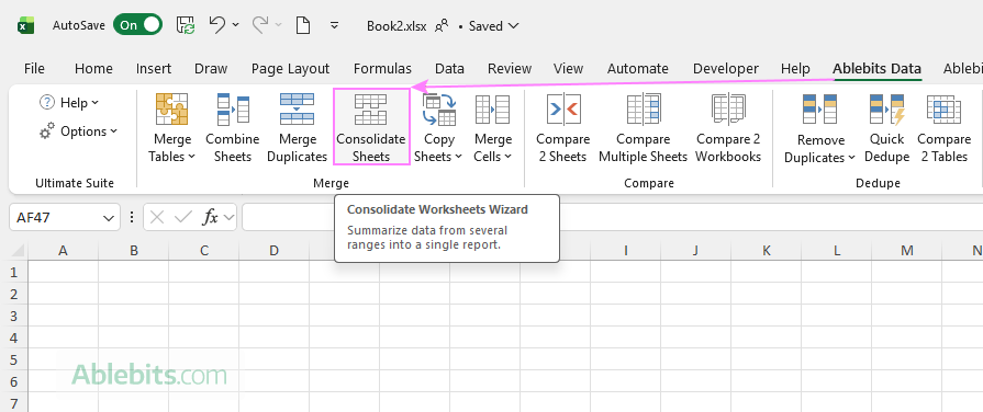
How to consolidate data in Excel in 3 simple steps:
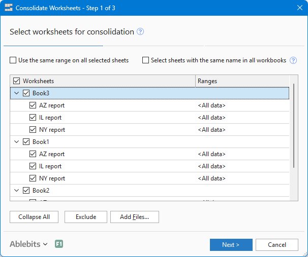
- Select files and sheets. The wizard shows all open workbooks and their worksheets in a user-friendly tree view, where you just tick the ones you want to include.
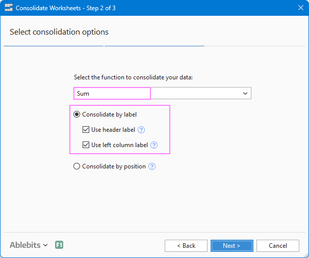
- Choose how to consolidate. Pick the summary function and decide whether the data should be matched by labels or by position.
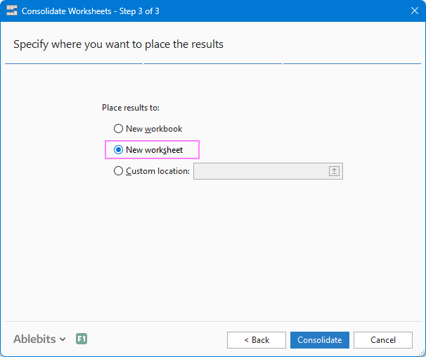
- Choose where to place the results. Specify where the consolidated data should appear: on a new workbook, new sheet, specific location in an existing sheet.
That's it. In just a few clicks, you get a well-organized summary in under a minute.
If you'd like to see how it works in practice, use the download link below to try it with your own data and explore its capabilities hands-on.
Thank you for reading, and I look forward to seeing you here again soon!
Available downloads
Consolidate data in Excel - examples (.xlsx file)
Ultimate Suite 14-day fully-functional version (.exe file)
 by
by