Today we'll discuss what you can do with dates and time in a Google spreadsheet. Let's take a closer look at how you can enter date and time into your table, and how to format and convert them to numbers.
How to insert date and time in Google Sheets
Let's start by entering the date and time into a Google Sheets cell.
Tip. Date and time formats depend on the default locale of your spreadsheet. To change it, go to File > Settings. You'll see a pop-up window where you can set your region under the General tab > Locale. Thus, you'll ensure those date and time formats you're accustomed to.
There are three ways to insert date and time into your Google spreadsheet:
Add date and time manually
Note. No matter how you want the time look like at the end, you should always enter it with a colon. This is essential for Google Sheets to distinguish between time and numbers.
It may seem to be the easiest way but locale settings that I mentioned above play a vital role here. Every country has its own pattern for displaying date and time.
As you all know, the American date format differs from the European one. If you set "United States" as your locale and type in the date in the European format: dd/mm/yyyy, it simply won't work. The entered date will be treated as a textual value. So, pay attention to that.
Tip. You can add today's date much quicker. Type @ in the required cells and continue with the word today:

Google Sheets will recognize your prompt and suggest you add Today's date. Click it, and your text will turn into today's date:

Confirm by pressing Enter.
Make Google Sheets auto-populate your column with date or time
Fill in a few cells with the required date/time/date time values.
Select these cells so you could see a small circle at the bottom right corner of the selection:
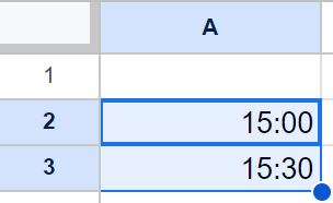
Click that circle and drag the selection down, covering all required cells.
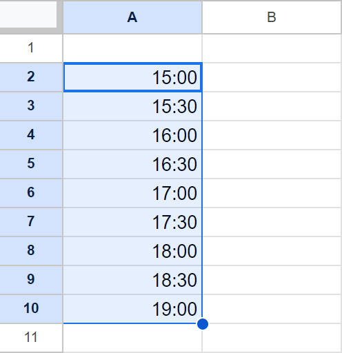
You'll see how Google Sheets automatically populates those cells based on two samples you provided, retaining the intervals:
Use key combinations to insert current date and time
Place the cursor into the cell of interest and press one of the following shortcuts:
- Ctrl+; (semicolon) to enter the current date.
- Ctrl+Shift+; (semicolon) to enter the current time.
- Ctrl+Alt+Shift+; (semicolon) to add both, current date and time.
Later you'll be able to edit the values. This method helps you bypass the problem of entering an incorrect date format.
Take advantage of Google Sheets date and time functions
TODAY() — returns the current date to a cell.
NOW() — returns the current date and time to a cell.
Note. These formulas will be recalculated, and the result will be renewed with every change made in the table.
Here you are: you've placed date and time to our cells. The next step is to format the information to display it the way you need it.
As it is with numbers, you can make your spreadsheet return date and time in various formats.
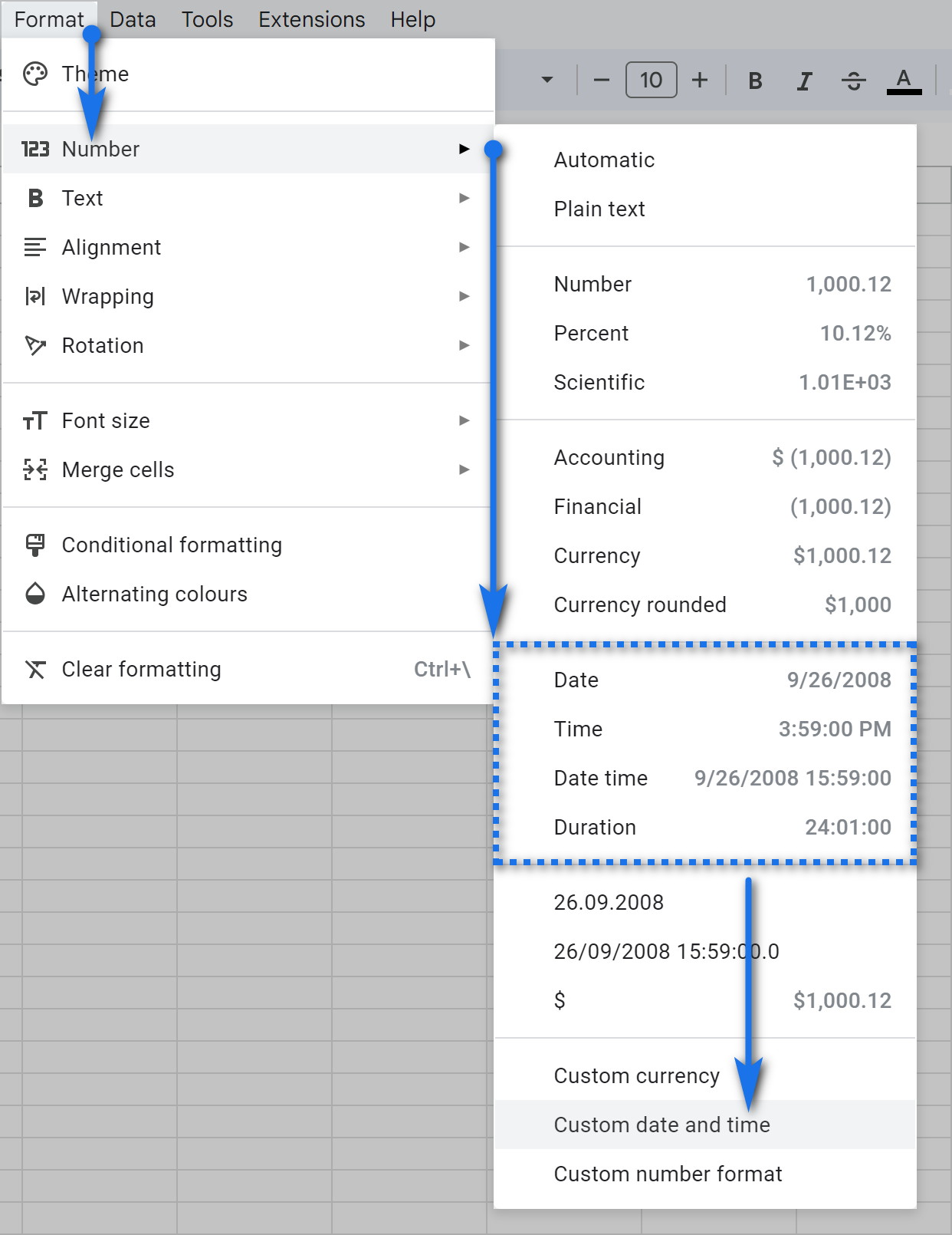
Place the cursor into the needed cell and go to Format > Number. You can choose between four different default formats or create a custom one using Custom date and time setting:
As a result, one and the same date looks different with various formats applied:
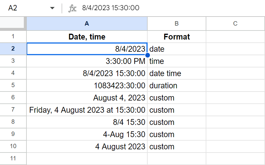
As you can see, depending on your needs, there are a few ways to set the date format. It allows displaying any date and time value, from a day to a millisecond.
Make your date/time a part of Data validation.
In case you need to use date or time in Data validation, proceed to Data > Data validation in the Google Sheets menu first:
- As for dates, just set them as criteria and choose the option that suits you best:
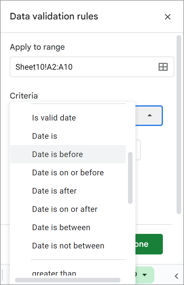
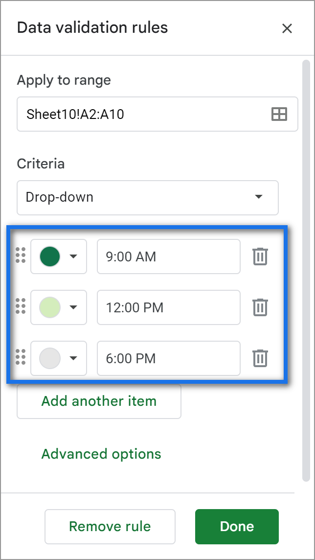
- As for time units, since they are absent from these settings by default, you will need to either create an additional column with time units and refer to this column with your Data validation criteria (List from a range), or enter time units directly to the criteria field (List of items) separating them by a comma:
Insert time to Google Sheets in a custom number format
Suppose you need to add time in minutes and seconds: 12 minutes, 50 seconds. Place the cursor to A2, type 12:50 and press Enter on your keyboard.
Note. No matter how you want the time to look like at the end, you should always enter it with a colon. This is essential for Google Sheets to distinguish between time and numbers.
What you'll see is Google Sheets treating your value as 12 hours 50 minutes. If you apply the Duration format to A2, it'll still show the time as 12:50:00.
So how can you make Google spreadsheet return only minutes and seconds?
- Type 00:12:50 to your cell.
To be honest, this one may turn out a tiresome process if you need to enter multiple timestamps with minutes and seconds only.
- Type 12:50 to A2 cell and put the following formula into A3:
=A2/60
Then apply the Duration number format to A3. Otherwise, your table will always return 12 hours AM. - Use special formulas.
Input minutes to A1, seconds — to B1. Enter the following formula to C1:
=TIME(0,A2,B2)
In order to delete excess symbols from our time, set the format again. Go to Custom date and time and create a format that will show only elapsed minutes and seconds:
The TIME function refers to cells, takes the values and transforms them into hours (0), minutes (A1), and seconds (B1).

Convert time to decimal in Google Sheets
Let's move on to various operations you can do with date and time in Google Sheets.
There may be cases when you need to display time as a decimal rather than "hh:mm:ss" to perform various calculations. Why? For example, to count per-hour salary, since you can't perform any arithmetic operations using both, numbers and time.
But the problem disappears if time is decimal.
Let's say column A contains the time you started working on some task and column B shows the end time. You want to know how much time it took, and for that, in column C you use the formula below:
=B2-A2
Copy the formula down cells C3:C5 and get the result in hours and minutes. Then transfer the values to column D using this formula:
=$C2
Then select entire column D and go to Format > Number > Number:

Unfortunately, the result you'll get at first won't say much. But Google Sheets has a reason for that: it displays time as a part of a 24-hour period. In other words, 50 minutes is 0.034722 of 24 hours.
Of course, this result can be used in calculations.
But since we're used to seeing time in hours, you may want to introduce more calculations to your table. To be specific, multiply the number you've got by 24 (24 hours):

Now you have a decimal value, where integer and fractional reflect the number of hours. To put it simply, 50 minutes is 0.8333 hours, while 1 hour 30 minutes is 1.5 hours.
Text-formatted dates to date format with Power Tools for Google Sheets
There's one quick solution for converting dates formatted as text to a date format. It's called Power Tools. Power Tools is an add-on for Google Sheets that allows you to convert your information in a couple of clicks:
- Install Power Tools to your Google Sheets by clicking the button below.
- Go to Extensions > Power Tools > Start to run the add-on and click the Convert tool icon on the add-on pane. Alternatively, you can pick the Tools > Convert tool right from the Power Tools menu.
- Select the range of cells that contain dates formatted as text.
- Check the box for the option Convert text to dates and click Run:
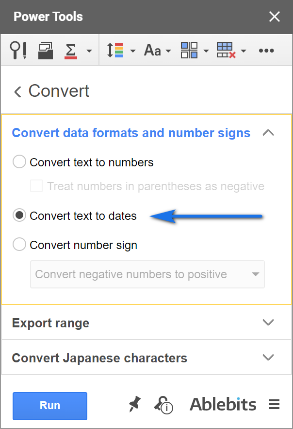
Your text-formatted dates will be formatted as dates in just a few seconds.
I hope you've learned something new today. If you have any questions left, feel free to ask them in the comments below.
Next time you'll learn how to calculate the time difference and sum dates and time together.
 by
by
98 comments
I want to store automatically date & time when data entered in sheets how can i do
Hello SPARTAN,
The functions mentioned here should help you.
This time only changes if you made changes to something but you can enter =NOW()
Can Google enter full dates (IE 2024-06-18) if I only enter the day and month, IE 18/6 for the 18th of June in the current year? Excel and OpenOffice both allow this. I'm wondering if Google Sheets does too. If so, how do I access this function, as at the moment, it's not doing so. BTW, I am in Australia, so 2024-06-18 instead of 2024-18-06.
Hello Dominic,
Yes, it can. First, you need to format cells as dates. Then enter 18/06 into these cells and they will appear in the required format.
hi!
can you help me with my google sheets
I want to show the cut-off date
for example, I want to show every 20th of the month
what formula will I use?
Hi ANN,
Sorry, could you please specify your task? Do you want the list of all months but only the 20th day? Or do you need to show 20th of each month when it's actually the 20th day? Or maybe for each previous month only?
i want day by day automatically date changing formula in google sheet
Hello vignesh,
Try the TODAY() function mentioned in this part of the article.
thanks a lot !!!
You're welcome :)
How to make one time can be select once only
Hello khairul,
I'm sorry but your question is not clear. Please describe your task in detail, I'll try to help.
Hello,
I am looking to create a descending list in column A for each month on each sheet/page.
I am trying to use a date format of: mm/dd/yy for each of the 12 pages, one for each month.
So, Column A1 would be the first day of that month, and A31 would be the last day of that month. One page per month. (I have the 12 pages/labels for the months figured out.)
Thank you for your time.
Hello Val,
Sorry, your question is not clear. Are you having difficulties entering the date units?
Are there any formulas in the Google sheets to know when and at what time did the google sheet got created and when and at what time it was last updated?
Currently i can see it only in the version history option. But i need to update the created date and time and last edited date and time information directly in the spreadsheet without checking in version history.
Thanks
Hello Bala,
I'm afraid Google Sheets doesn't have formulas for this. You may try to find a solution here – an overview of Google Apps Script with a lot of helpful content and links: https://developers.google.com/apps-script/overview
I hope you’ll find this information helpful. Sorry I can't assist you better.
Hello,
I opened a csv file with google sheets and there are a lot of dates like this one 9/29/2022, 10:04:04 PM (mm/dd/yyyy hh:mm:ss am/pm). This csv file i have to import it in a program wich read the dates dd/mm/yyyy hh:mm:ss am/pm and at dates like this 9/29/2022, 10:04:04 PM it show error "invalid date" . Is possible to change 9/29/2022 in 29/09/2022 without doing this manually (too many dates to change manually) ?
Hello Lenovo,
Try changing the locale in the file uploaded to Google Sheets first.
If this doesn't help, try applying the new custom format to all dates at once by these instructions.
Yet all these are still manual. To do this automatically, you'd have to use Google Apps Script.
HI... i want to record the time when a specific event (e.g., "Permission") occurs in cell G, and display the time in cells H & another event occurs (e.g., "Return") and display the time in cells J, & Assuming i want to calculate the time duration in cell k.
Hi ranjith kumar,
I believe Khawaja Arshad below shared the solution for the same task.
Hello Natalia,
I am trying to create a formula where "IF Date is "Today" Then, "Due Today" type of statement.
Additionally, "If Date is "Past Due" Then,"Assignment Overdue" ...
Not sure exactly how to put this together or if it is possible.
Im actually looking to insert this into a "Monday.com" formula box but this should also be universal with the formula structures in Google.
Thanks in advance.
Hi! To get a value by condition, use these guidelines: Google Sheets IF function – usage and formula examples. If I understand your task correctly, try the following formula:
=if(A1=today(), "Today",if(A1<today(),"Assignment Overdue",""))
I am trying to validate a complete date in google sheets, and have been using the "isDate()" function. However, it validates true even if the date is just a month/year although all the documentation I've seen says that it requires a month/day/year. Is there a way to validate that a cell and require the month, day and year? It seems that it just defaults to the first day of the month.
Ex: Cell A1 contains "10/1929"
=isDate(A1) returns true
=Day(A1) returns 1
Hello Mitch,
Google Sheets picks up dates written in different formats. Hence, you're right, it treats 10/1929 as October 1st, 1929. You'll see the same in the formula bar if you select the cell. I'm afraid this is a matter of the format visible to you which cannot be handled with formulas.
However, you can try some kind of a workaround. For example, use the IF function to check if the Day from A1 equals 1. And if so, mark the date as potentially incomplete.
how to insert drop down date and time in one chell
Hello Padmanaban,
Please check out this article: How to add, edit and delete drop-down lists in Google Sheets
I have a sheet with contacts from different time zones within the US. How can I show the time zone of each contact? is there a way to convert time to different time zone so I can have a single time for every contact?
Hello Nasir Khan,
I'm afraid there are no standard functions to work with the time zones. You will have to add formulas that add the required amount of hours to show the same time zone for each contact.
Alternatively, you can use scripts. You may try to find the solution here – an overview of Google Apps Script with a lot of helpful content and links: https://developers.google.com/apps-script/overview
I am using google sheet and applying formula =IF(L2="Fully Consumed",TODAY(),""), it means that if condition is fulfilled in L2 Column i.e. "Fully Consumed" then Current Date should be in N2 columns, it is applying properly but Date is changed on daily basis as current date which should not be done, I want that date should be applied once then should not be changed as date changed. Is there any proper solution of my problem?
Hello Khawaja Arshad,
TODAY is a volatile function meaning it recalculates itself in all cells once anything at all is edited in your spreadsheet. Since there are no other standard formulas for this task, I can advise you to either replace dates with values at the end of the day or use scripts. You may try to find the solution here – an overview of Google Apps Script with a lot of helpful content and links: https://developers.google.com/apps-script/overview
Hello There,
I need to enter the same date for 5 rows (2023-06-12) and then the next day for the next 5 rows (2023-06-13), etc, etc. The sheet is configured to follow date order when it is dragged down. I have tried manually adding about 15 rows (3 dates) and then dragging down, but it still converts backs to putting one day in each row. Please help! Thanks :)
Hello Susan,
Here's what you can do:
Use the dragging on steps 1-3 to speed up the process. It'll be much quicker than entering dates by groups one by one.
Thanks for answering so quickly, Unfortunately, this did not work the way I need it to. I ended up with just 3 coloumns on a new spreadsheet ( so all the other data was missing, and the dates ended up like this...
2023-05-08
2023-05-09
2023-05-10
2023-05-11
2023-05-09
2023-05-10
2023-05-11
2023-05-12
2023-05-10
where as I need.....
2023-05-08
2023-05-08
2023-05-08
2023-05-08
2023-05-09
2023-05-09
2023-05-09
2023-05-09
2023-05-10
Thanks!
We need to input today's date using a tablet or phone, entering business incomes/transaction.
On the computer ctrl+; works great, but how to do this on a tablet, iPad specifically?
Hello Genadi,
You can use shortcuts on iPad only if you connect an external keyboard to your iPad: https://support.google.com/docs/answer/181110?hl=en&co=GENIE.Platform%3DiOS&oco=0#zippy=%2Cmac-shortcuts
I WANT THE RESULT IN THE SPECIFIED CELL AFTER SPECIFIC TIME.
HOW TO GET IT.
MEANS,
=A1+A2
IS FORMULA WRITTEN IN A3 BUT THE RESULT IN A3 MUST BE VISIBLE SAY AFTER 5 MINUTES (SPECIFIC TIME AND NOT IMMEDIATLY. HOW TO GET IT??
Hello CHAKOR,
I'm afraid it's impossible with the standard Google Sheets functions. You need to use a script for the task. Since we do not cover the programming area (script-related questions), I can suggest looking for a solution here – an overview of Google Apps Script with a lot of helpful content and links:
https://developers.google.com/apps-script/overview
I hope you’ll find this information helpful. Sorry I can't assist you better.
This worked =TODAY()
Thank you.
You're most welcome, we're glad the article helped! :)
Hi what is the formula of this,? when inserting data in A1 the A2 automatic date and time that did not change when I open tom.. Because when I encode tom. the date and time is automatic update
Hello Marseille,
I'm sorry, your question is not clear. Please describe the problem in detail, I'll try to help.
I am creating a spreadsheet for my online classmates.
We are all over the world, and I am wondering if there is a way to have a cell show what time it is in each person's locale (updating itself every minute to the current time). Can I tell the cell to show current Eastern Standard time in one cell, and current Swedish time in another cell?
Hello kargelc,
If you're in Eastern Standard Time, set this time zone in your spreadsheet settings first. Then =NOW() will show your current time.
Swedish is located 5 hours away from EST. So use =NOW() + 5/24 to show Swedish time in another cell.
Hello!
I am looking to have a date pop into a separate column, when a checkbox is marked complete
For example checkbox is in column C, i have completed my task and once i check the box, todays date would pop into Column E
Thank you for your help!
Hello Wilfredo,
You need to use the IF function along with TODAY. However, TODAY is a volatile function. It recalculates itself in all cells each time anything is edited somewhere on the sheet. There are a few workarounds to this: