Quick features of the smart toolbar

Power Tools sidebar offers a smart toolbar at the top for the most common operations. Each operation is available at a single click, with optional drop-down lists next to the default action. The only exceptions are Advanced Find and Replace, Function by Color and Sheets Manager: the tools take the entire sidebar with their settings. Sort by Color offers both the options in the drop-down as well as sidebar with advanced settings.

• How to work with smart toolbar
  • Start Power Tools
  • Search and replace data in Google Sheets
  • Count and sum values by fill and font color
  • Easily manage multiple sheets
  • Sort by color in Google Sheets
  • Change case in Google Sheets
  • Remove empty rows and columns
  • Freeze panes in a Google spreadsheet
  • Calculate numbers in the selected columns or rows
  • Unpivot table in Google Sheets
  • Flip cells, columns, or rows in a Google spreadsheet
  • Unmerge cells in a spreadsheet

How to work with smart toolbar

Start Power Tools

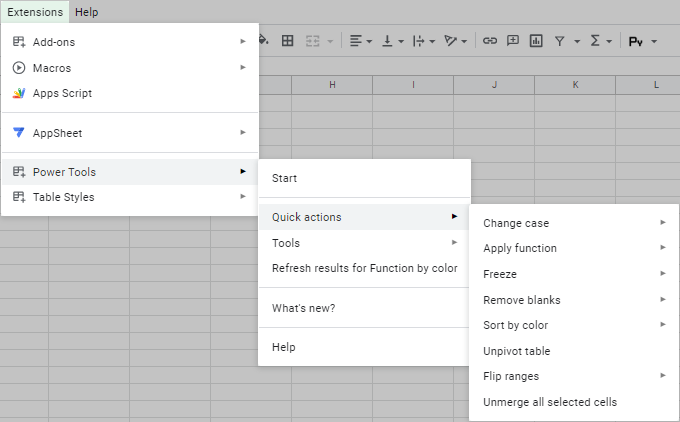
Go to Extenstions > Power Tools > Start to open the add-on in Google Sheets:

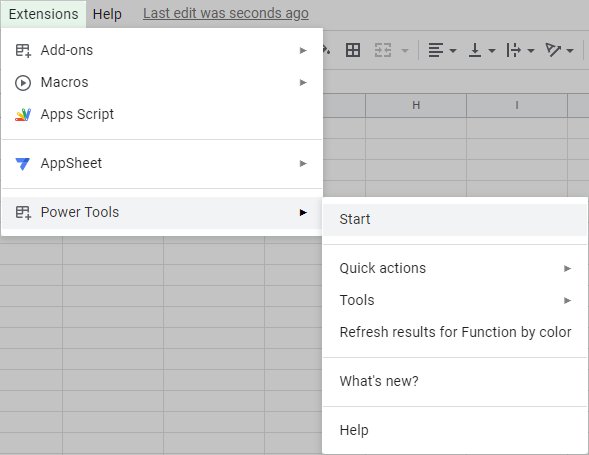
You will see the Power Tools sidebar with the toolbar options right at its top.

Tip. You can run some of the Smart Toolbar add-ons directly from the Google Sheet menu: Extensions > Power Tools > Quick actions:

Search and replace data in Google Sheets

This two-step add-on performs a comprehensive search in the selected sheets, shows the list with the results, and allows you to browse, export, or replace the found entries:

Learn how to find and replace data in your sheets.

Count and sum values by fill and font color

Function by Color allows you to calculate records formatted in a certain way in any range.

Learn how to calculate cells by their colors.

Easily manage multiple sheets

Sheets Manager is the most convenient and friendly-user way to see, select & handle sheets in bulk: hide sheets, lock, color, reorder, etc.

Learn how to easily manage several sheets.

Sort by color in Google Sheets

Though Google Sheets has its tool to sort by color, this utility offers sorting by colors from another angle. It sorts either your selected range or the entire sheet by the fill or font colors they contain.

Learn how to sort by color in Google Sheets.

Change case in Google Sheets

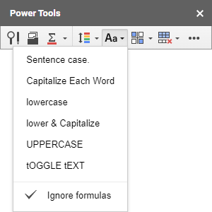
This one is the shortcut to changing cases in all cells of interest.

First, tick off the Ignore formulas option if you want to prevent all formulas you may have from turning into values. The tool won't process such cells at all.

Then, select the necessary data in your spreadsheet, click on the tool's icon, and choose one of 6 cases:

Remove empty rows and columns

Select any cell in your table, click the tool icon and hit whatever you want to get rid of:

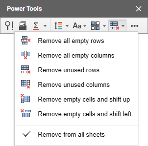
• The first two options will delete all completely blank lines and columns inside your table.
• The next two actions will deal with blank lines and columns outside of your table.
  Tip. Remove unused rows and columns to contribute to spare cells in your spreadsheet and make it harder to reach the Google Sheets limit for 5 million cells. Also, this will speed up data processing.
• The last one, if ticked off, will make sure to remove all empty and unused rows and columns from all sheets in the spreadsheet.

Freeze panes in a Google spreadsheet

• To leave the header rows and left columns visible when scrolling in large tables, select a cell right under and to the right of the area you want to remain visible and click the icon with three dots and then the Freeze panes icon:
  
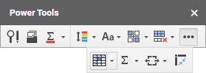
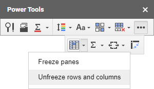
  This will lock all rows above and columns to the left of the selected cell.
• To unfreeze rows and columns, click on the down arrow next to Freeze pane and pick Unfreeze rows and columns:
  

Calculate numbers in the selected columns or rows

The utility lets you get the formulas for the most common functions in a click. Even if you have multiple columns with numbers, simply select empty cells under those columns. The add-on will quickly process the data in each column and paste the correct result to each corresponding empty cell.

1. Select columns with numbers that you want to count.
   Tip. You can highlight a blank column next to rows of numbers to add calculations to each row.
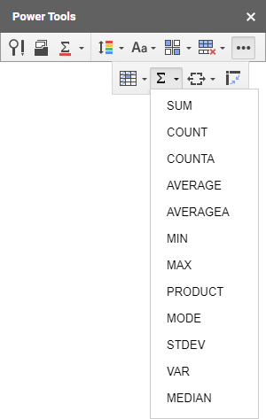
2. Click on the icon with three dots to see more tools, then hit the Calculate tool, and pick one of 12 functions to add its formula under each column:
   

Unpivot table in Google Sheets

Use this tool to normalize a pivot table and get a flat list instead.

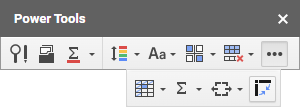
Select the range with your crosstab table, click the icon with three dots on the Power Tools smart toolbar, then on the Unpivot Table icon itself, and have the resulting database list pasted to a new spreadsheet:

Flip cells, columns, or rows in a Google spreadsheet

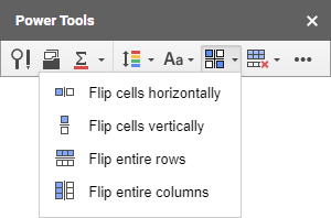
Supposedly a simple task of flipping two adjacent cells involves a lot of copying and pasting. The Flip tool allows you to do this in just two clicks:

1. Select adjacent cells you want to switch contents between.
   Tip. To exchange data between rows or columns, you don't have to highlight the entire rows or columns: selecting cells from them and picking the options to flip entire rows/columns is enough.
2. Click the Flip icon and pick the necessary option from the drop-down list:
   

Unmerge cells in a spreadsheet

Last but not least is the little assistant that helps you unmerge cells. You'll find it if you click the icon with three dots on the toolbar:

• To unmerge all selected cells, highlight the range that contains them and either click on the tool's icon or click on the down arrow next to the icon and pick the first option from the drop-down menu.
• To unmerge all cells on the sheet, select any cell on the spreadsheet of interest, click on the down arrow next to the icon, and pick the second option from the drop-down menu.