In this tutorial, you will learn a few quick and efficient ways to check and debug formulas in Excel. See how to use the F9 key to evaluate formula parts, how to highlight cells that reference or are referenced by a given formula, how to determine mismatched or misplaced parentheses, and more.
In the last few tutorials, we have been investigating different aspects of Excel formulas. If you've had a chance to read them, you already know how to write formulas in Excel, how to show formulas in cells, how to hide and lock formulas, and more.
Today, I'd like to share a few tips and techniques to check, evaluate and debug Excel formulas that will hopefully help you work even more efficiently with Excel.
F2 key in Excel - edit formulas
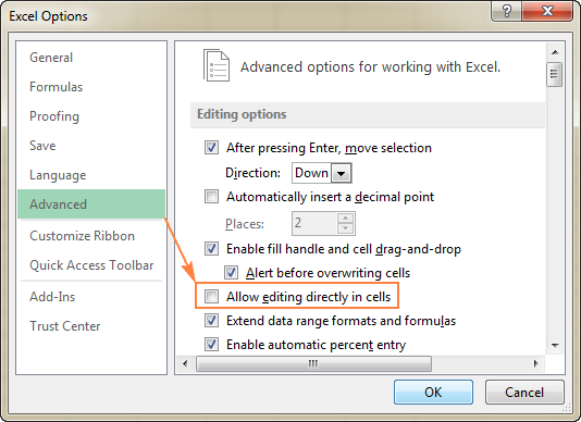
The F2 key in Excel toggles between Edit and Enter modes. When you want to make changes to an existing formula, select the formula cell and press F2 to enter the Edit mode. Once you do this, the cursor starts flashing at the end of the closing parenthesis in the cell or formula bar (depending on whether the Allow editing directly in cells option is checked or unchecked). And now, you can make any edits in the formula:
- Use the left and right arrows to navigate within the formula.
- Use the arrow keys together with Shift to select the formula parts (the same can be done using the mouse).
- Press Delete or Backspace to delete certain cell references or other elements of the formula.
When you are done editing, press Enter to complete the formula.
To exit the Edit mode without making any changes to the formula, press the Esc key.
Editing directly in a cell or in the formula bar
By default, pressing the F2 key in Excel positions the cursor at the end of the formula in a cell. If you prefer editing formulas in the Excel formula bar, do the following:
- Click File > Options.
- In the left pane, select Advanced.
- In the right pane, uncheck the Allow editing directly in cells option under Editing Options.
- Click OK to save the changes and close the dialog.
These days, F2 is often considered an old-fashioned way to edit formulas. Two other ways to enter the Edit mode in Excel are:
- Double clicking the cell, or
- Clicking anywhere within the formula bar.
Is Excel's F2 approach more efficient or does it have any advantages? Nope :) Simply some people prefer working from the keyboard most of the time while others find it more convenient to use the mouse.
Whichever editing method you choose, a visual indication of the Edit mode can be found at the bottom-left corner of the screen. As soon as you press F2, or double click the cell, or click the formula bar, the word Edit will appear right below the sheet tabs:

Tip. Press Ctrl + A to jump from editing a formula in a cell to the formula bar. It only works when you are editing a formula, not a value.
F9 key in Excel - evaluate formula parts
In Microsoft Excel, F9 key is an easy and quick way to check and debug formulas. It lets you evaluate only the selected part of the formula by replacing it with the actual values that part operates on, or with the calculated result. The following example demonstrates Excel's F9 key in action.
Supposing you have the following IF formula in your worksheet:
=IF(AVERAGE(A2:A6)>AVERAGE(B2:B6),"Good","Bad")
To evaluate each of the two Average functions included in the formula individually, do the following:
- Select the cell with the formula, D1 in this example.
- Press F2 or double click the selected cell to enter the Edit mode.
- Select the formula part you want to test and press F9.
For example, if you select the first Average function, i.e. AVERAGE(A2:A6), and press F9, Excel will display its calculated value:
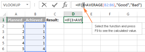
If you select only the cell range (A2:A6) and press F9, you will see the actual values instead of the cell references:

To exit the formula evaluation mode, press the Esc key.
Excel F9 tips:
- Be sure to select some part of your formula before pressing F9, otherwise the F9 key will replace the entire formula with its calculated value.
- When in the formula evaluation mode, don't press the Enter key because this would replace the selected part either with the calculated value or cell values. To retain the original formula, press the Esc key to cancel the formula testing and exit the formula evaluation mode.
The Excel F9 technique is especially useful for testing long complex formulas, such as nested formulas or array formulas, where it's difficult to understand how the formula calculates the final result because it includes a few intermediate calculations or logical tests. And this debugging method lets you narrow down an error to a particular range or function causing it.
Debug a formula by using the Evaluate Formula feature
Another way to evaluate formulas in Excel is the Evaluate Formula option that resides on the Formulas tab, in the Formula Auditing group.

As soon as you click this button, the Evaluate Formula dialog box will pop up, where you can inspect each part of your formula in the order the formula is calculated.
All you need to do is click the Evaluate button and examine the value of the underlined formula part. The result of the most recent evaluation appears in italics.
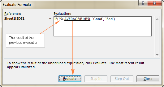
Continue clicking the Evaluate button until each part of your formula has been tested.
To end the evaluation, click the Close button.
To start the formula evaluation from the beginning, click Restart.
If the underlined part of the formula is a reference to a cell containing another formula, click the Step In button to have that other formula displayed in the Evaluation box. To get back to the previous formula, click Step Out.
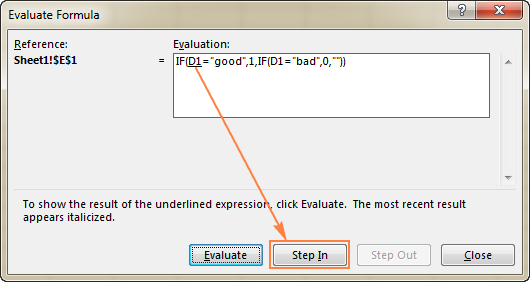
Note. The Step In button is not available for a cell reference pointing to another formula in a different workbook. Also, it is not available for a cell reference that appears in the formula for the second time (like the second instance of D1 in the screenshot above).
Highlight and match parenthesis pairs in a formula
When creating sophisticated formulas in Excel, you often need to include more than one pair of parentheses to specify the order of calculations or nest a few different functions. Needless to say, it's very easy to misplace, omit, or include an extra parenthesis in such formulas.
If you miss or misplace a parenthesis and hit the Enter key attempting to complete the formula, Microsoft Excel usually displays an alert suggesting to fix the formula for you:
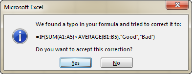
If you agree to the suggested correction, click Yes. If the edited formula is not what you want, click No and make the corrections manually.
Note. Microsoft Excel does not always fix missing or mismatched parentheses correctly. Therefore, always review the proposed correction carefully before accepting it.
To help you balance the parenthesis pairs, Excel provides three visual clues when you are typing or editing a formula:
- When entering a complex formula that contains multiple sets of parenthesis, Excel shades parenthesis pairs in different colors to easier identify them. The outside parenthesis pair is always black. This can help you determine whether you have inserted the right number of parenthesis in your formula.
- When you type the closing parenthesis in a formula, Excel briefly highlights the parenthesis pair (the right parenthesis you've just typed and the matching left parenthesis). If you've typed what you think is the last closing parenthesis in a formula and Excel doesn't bold the opening one, your parentheses are mismatched or unbalanced.
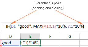
- When you navigate within a formula using the arrow keys and cross over a parenthesis, the other parenthesis in the pair gets highlighted and formatted with the same color. In this way, Excel tries to make parenthesis pairing more evident.
In the following screenshot, I've crossed over the last closing parenthesis using the arrow key, and the outside parenthesis pair (black ones) got highlighted:
Highlight all cells referenced in a given formula
When you are debugging a formula in Excel, it might be helpful to view the cells referenced in it. To highlight all of the dependent cells, do the following:
- Select the formula cell and press the Ctrl + [ shortcut. Excel will highlight all the cells your formula refers to, and moves the selection to the first referenced cell or a range of cells.
- To navigate to the next referenced cell, press Enter.
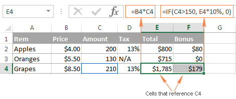
In this example, I selected cell F4 and pressed Ctrl + [ . Two cells (C4 and E4) referenced in F4's formula got highlighted, and the selection moved to C4:

Highlight all formulas that reference a selected cell
The previous tip demonstrated how you can highlight all the cells referenced in a certain formula. But what if you want to do the reverse and find out all the formulas that refer to a particular cell? For example, you might want to delete some irrelevant or outdated data in a worksheet, but you want to make sure the deletion won't break any of your existing formulas.
To highlight all cells with formulas that reference a given cell, select that cell, and press the Ctrl + ] shortcut.
Like in the previous example, the selection will move to the first formula on the sheet that references the cell. To move the selection to other formulas that reference that cell, press the Enter key repeatedly.
In this example, I've selected cell C4, pressed Ctrl + ] and Excel immediately highlighted the cells (E4 and F4) containing a C4 reference:
Trace relationships between formulas and cells in Excel
Another way to visually display cells relating to a certain formula is to use the Trace Precedents and Trace Dependents buttons that reside on the Formulas tab > Formula Auditing group.
Trace Precedents - show cells that supply data to a given formula
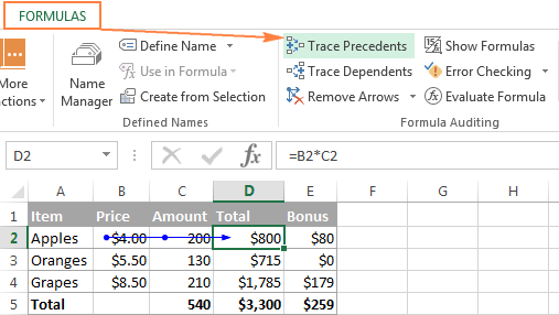
The Trace Precedents button works similarly to the Ctrl+[ shortcut, i.e. shows which cells provide data to the selected formula cell.
The difference is that the Ctrl + [ shortcut highlights all cells referenced in a formula, while clicking the Trace Precedents button draws blue trace lines from the referenced cells to the selected formula cell, as demonstrated in the following screenshot:
To get precedents lines to appear, you can also use the Alt+T U T shortcut.
Trace Dependents - show formulas that reference a given cell
The Trace Dependents button works similarly to the Ctrl + ] shortcut. It shows which cells are dependent on the active cell, i.e. which cells contain formulas referencing a given cell.
In the following screenshot, cell D2 is selected, and the blue trace lines point to the formulas that contain D2 references:
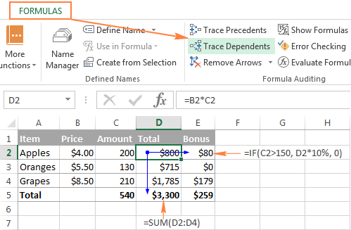
Another way to display dependents line is clicking the Alt+T U D shortcut.
Tip. To hide the trace arrows, click the Remove Arrows button that resides right belowTrace Dependents.
Monitor formulas and their calculated values (Watch Window)
When you are working with a large data set, you may want to keep an eye on the most important formulas in your workbook and see how their calculated values change when you edit the source data. Excel's Watch Window was created just for this purpose.
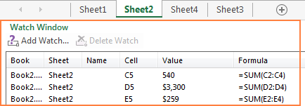
The Watch Window displays the cell properties, such as the workbook and worksheet names, cell or range name if any, cell address, value, and formula, in a separate window. In this way, you can always see the most important data at a glance, even when you are switching between different workbooks!
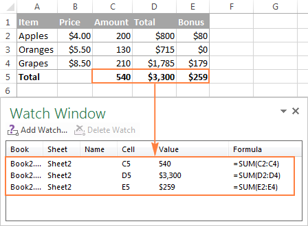
How to add cells to the Watch window
To display the Watch Window and add cells to monitor, perform the following steps:
- Select the cell(s) that you want to watch.
Tip. If you want to monitor all the cells with formulas on an active sheet, go to the Home tab > Editing group, click Find & Replace, then click Go To Special, and select Formulas.
- Switch to the Formulas tab > Formula Auditing group, and click Watch Window.

- The Watch Window will appear and you click the Add Watch… button.
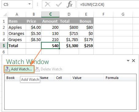
Watch Window notes:
- You can add only one watch per cell.
- Cells that have external references to other workbook(s) are displayed only when those other workbooks are open.
How to remove cells from the Watch Window
To delete a certain cell(s) from the Watch Window, select the cell you want to remove, and click the Delete Watch button:
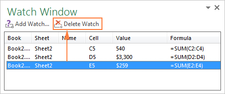
Tip. To delete several cells in one go, press Ctrl and select the cells you want to remove.
How to move and dock the Watch Window
Like any other toolbar, Excel's Watch Window can be moved or docked to the top, bottom, left, or right side of the screen. To do this, just drag the Watch Window using the mouse to the location you want.
For example, if you dock the Watch Window to the bottom, it will always show up just below your sheet tabs, and let you comfortably inspect the key formulas without having to repeatedly scroll up and down to the formula cells.
And finally, I'd like to share a couple more tips that might prove helpful for evaluating and debugging your Excel formulas.
Formula debugging tips:
- To view a long formula entire without overlaying the contents of neighboring cells, use the formula bar. If the formula is too long to fit into the default formula bar, expand it by pressing Ctrl + Shift + U or drag its lower border using the mouse as demonstrated in How to expand the formula bar in Excel.
- To see all formulas on the sheet instead of their results, press Ctrl + ` or click the Show Formulas button on the Formulas tab. Please see How to show formulas in Excel for full details.
This is how to evaluate and debug formulas in Excel. If you know more efficient ways, please do share your debugging tips in comments. I thank you for reading and hope to see you on our blog next week!
 by
by
9 comments
Hello and thanks for such huge help
I have a formula in excel which has some refrences in other sheets
but when I choose the formula bar, the cells in other sheets are not highlighted and seems not to have any connection between them and formula
what do you recommend me about it
?
Hi! When you edit a formula, only the cells on the current sheet are highlighted. Try using the Trace Precedents tool as described in this tutorial: How to trace relationships between formulas and cells.
=IF(K4>1,G4*1.1), IF(K4>2,G4*1.21)
Please i Need this if any solution i want to create but i have an idea how is formula work
I can't guess what result you want to get, but maybe this formula will work for you:
=IF(IF(K4>2,G4*1.21, K4>1,G4*1.1))
Thanks a lot!
Did you miss one for the keyboard lovers? Ctrl + A to jump from the formula edit within the cell into the formula bar (only works if you have a formula, not with a value)
Hi Jo,
Yep, I missed that. Just added this tip to the article. Thank you!
Hello Svetlana,
Hope you are doing well.
Is there a formula to get only the year from a full date, e.g. we have the date 01-Feb-16 and we need to get the year "2016" in the cell next to date.
Warm Regards,
Suliman
Hi Suliman,
Sure, you can use the YEAR function for this. The formula can be as simple as =YEAR(A1) where A1 is a full date.
Hi Svetlana,
Thank you very much.