The IF function in Google Sheets is one of the easiest functions to learn, and while this holds true, it is also a very helpful one.
In this tutorial, I invite you to take a closer look at how Google Spreadsheet IF function works and what advantages you will get from using it.
What is the IF function in Google Sheets?
Whenever you use the IF function, you create a decision tree in which certain action follows under one condition, and if that condition is not met – another action follows.
For this purpose, the condition of the function must be in a format of the alternative question with only two possible answers: "yes" and "no".
This is what a decision tree may look like:
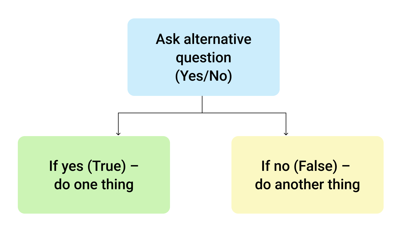
So, the IF function allows you to ask a question and indicate two alternative actions depending on the received answer. This question and the alternative actions are known as three arguments of the function.
IF function syntax in Google Sheets
The syntax for the IF function and its arguments are as follows:
- logical_expression – (required) a value or logical expression that is tested to see if it is TRUE or FALSE.
- value_if_true – (required) the operation that is carried out if the test is TRUE.
- value_if_false – (optional) the operation that is carried out if the test is FALSE.
Let's explore the arguments of our IF function in more detail.
The first argument represents a logical question. Google Sheets answers this question with either "yes" or "no", i.e. "true" or "false".
How to formulate the question properly, you may wonder? To do that, you can write a logical expression using such helpful symbols (or comparison operators) as "=", ">", "<", ">=", "<=", "<>". Let us try and ask such a question together.
Usage of the IF function
Let's assume that you are working in the company selling chocolate in several consumer regions with many clients.
This is what your sales data may look like in Google Sheets:
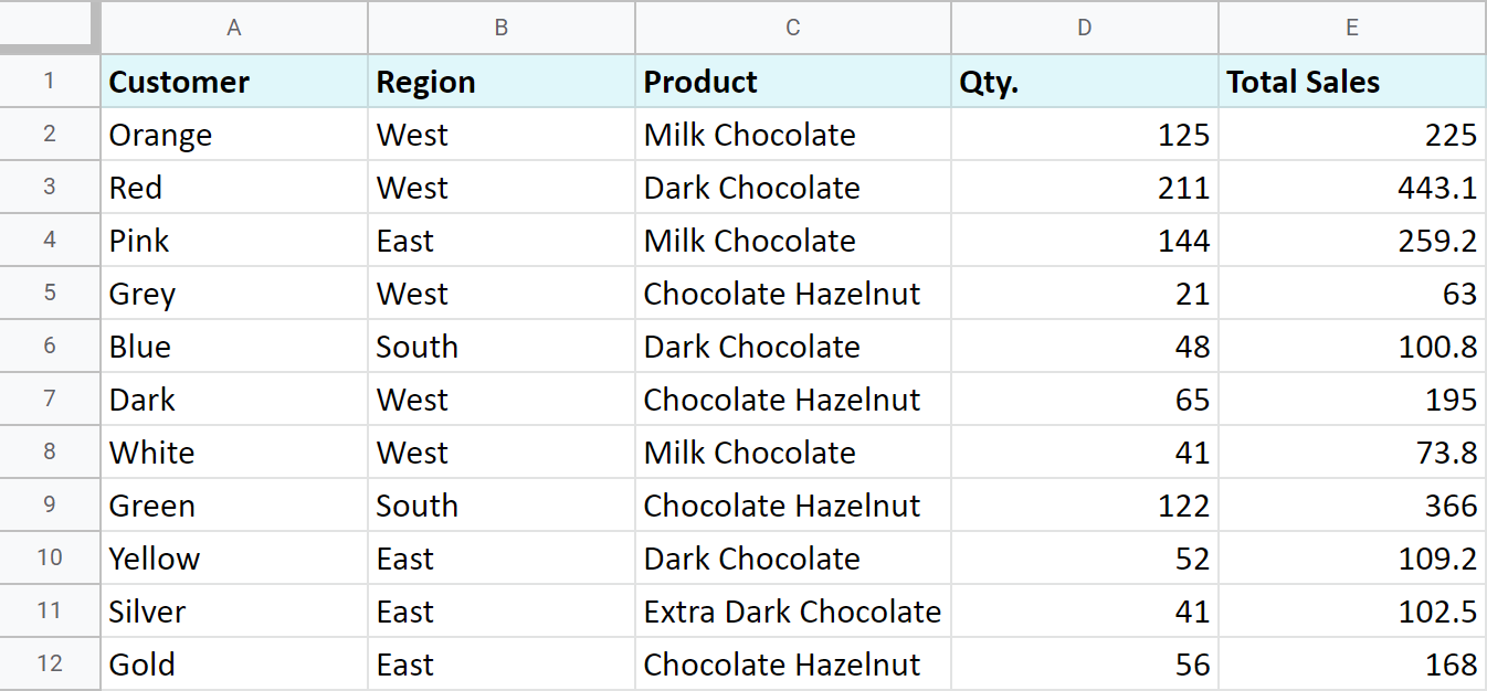
Imagine that you need to separate sales made in your local regions from those from abroad. To accomplish that, you should add another descriptive field for each sale – a country where the sales took place. Since there is a lot of data, you need this description field to be created automatically for each entry.
And this is when the IF function comes to play. Let's add the "Country" column to the data table. "West" region represents local sales (Our Country), while the rest are the sales from abroad (Rest of the World).
How to write out the function properly?
Place the cursor in F2 to make the cell active and type in the equality sign (=). Google Sheets will immediately understand that you are going to enter a formula. That's why right after you type the letter "i" it will prompt you to choose a function that begins with that same letter. And you should choose "IF".
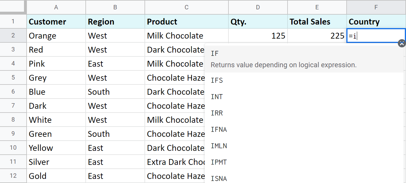
After that, all your actions will be accompanied by prompts as well.
For the first argument of the IF function, enter B2="West". As with the other Google Sheets functions, you don't need to enter the address of the cell manually – a mouse click is enough. Then enter comma (,) and specify the second argument.
The second argument is a value that F2 will return if the condition is met. In this case, it will be the text "Our Country".
And again, after the comma, write the value of the 3rd argument. F2 will return this value if the condition is not met: "Rest of the World". Do not forget to finish your formula entry by closing parenthesis ")" and pressing "Enter".
Your entire formula should look like this:
=IF(B2="West","Our Country","Rest of the World")
If everything is correct, F2 will return the text "Our Country":
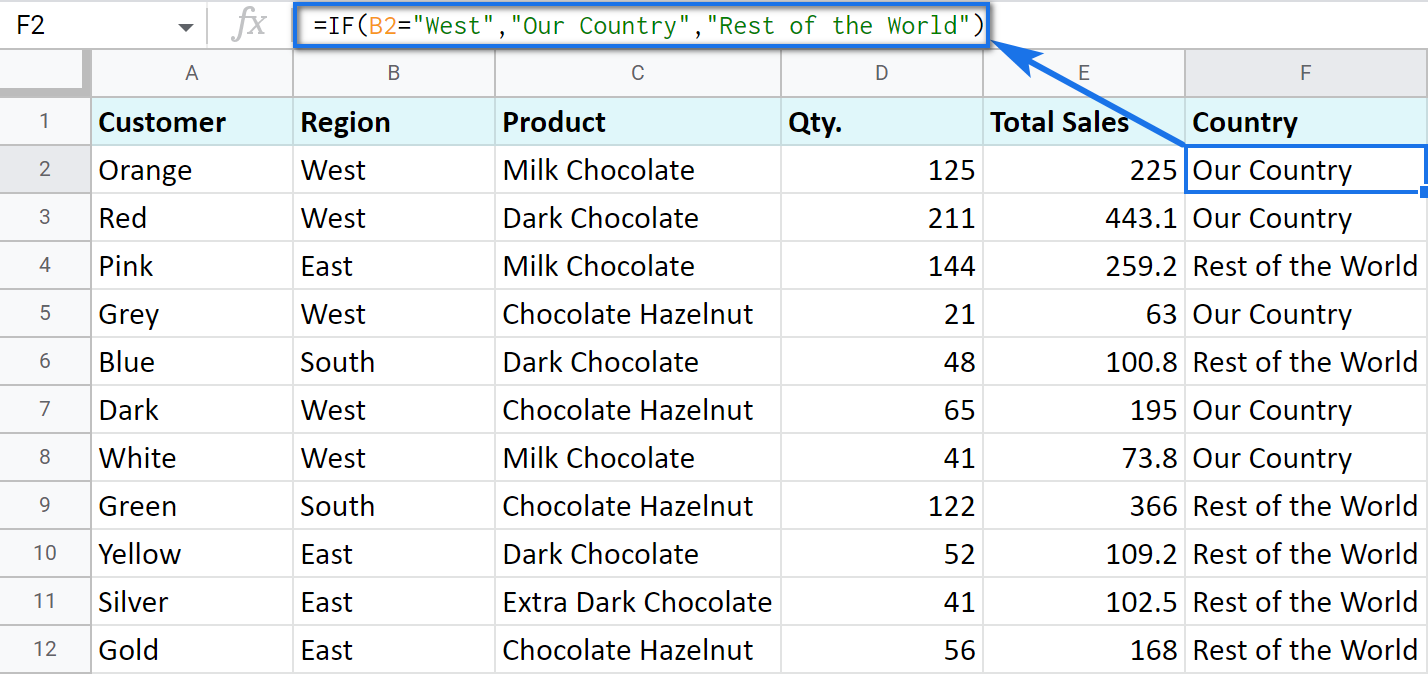
Now, all you have to do is to copy this function down column F.
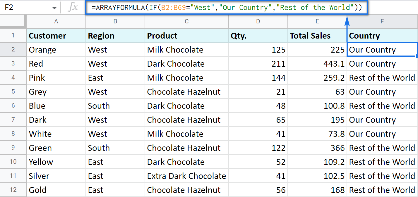
Tip. There's one way to process the entire column with one formula. The ARRAYFORMULA function will help you do that. Using it in the first cell of the column, you can test all cells below against the same condition, and return the corresponding result to each row at the same time:
=ARRAYFORMULA(IF(B2:B69="West","Our Country","Rest of the World"))
Let's examine the other ways of working with the IF function.
IF function and text values
The usage of the IF function with a text has already been illustrated in the example above.
Note. If the text is being used as the argument, then it must be enclosed in double-quotes.
IF function and numerical values
You can use numbers for the arguments just as you did with the text.
However, what is very important here is that the IF function makes it possible to not only fill cells with certain numbers based on the conditions met but also calculate.
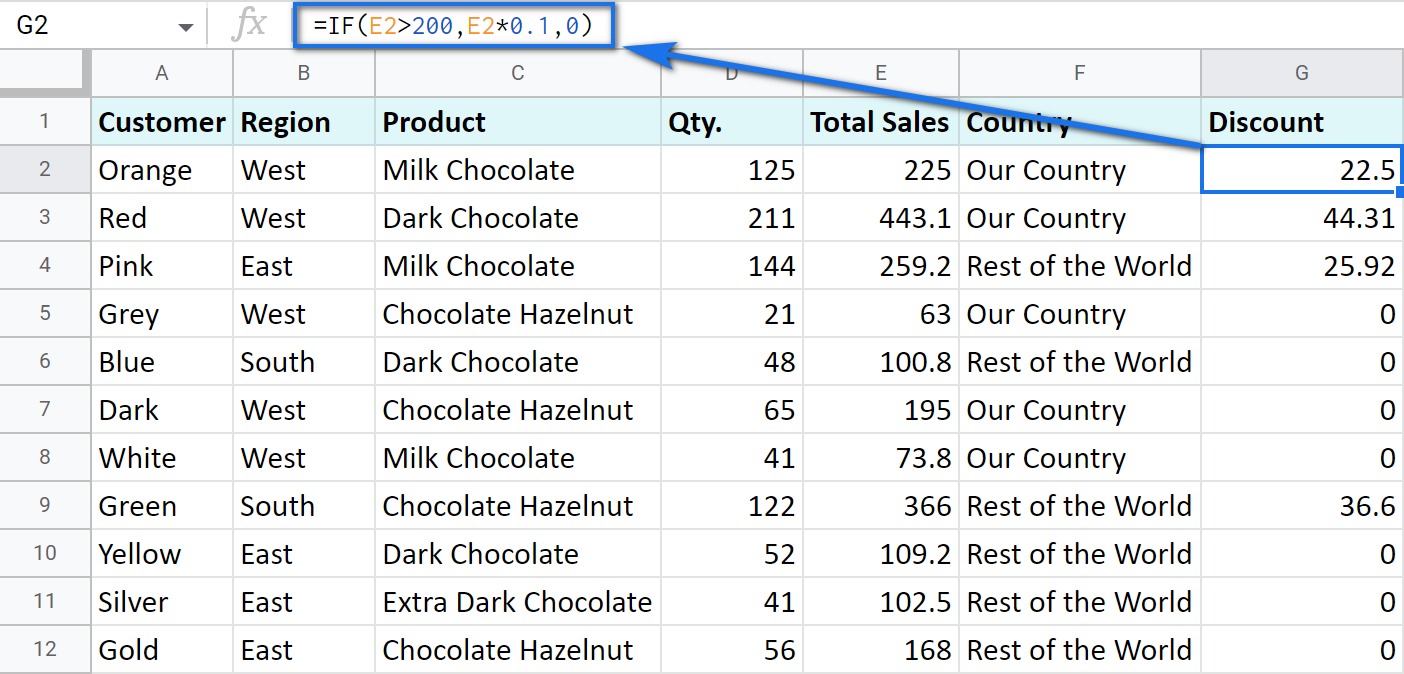
For example, let's say you offer your clients various discounts based on the total value of the purchase. If the total is more than 200, then the client gets a 10% discount.
For that, you need to use column G and name it "Discount". Then enter the IF function in G2, and the second argument will be represented by the formula that calculates the discount:
=IF(E2>200,E2*0.1,0)
IF blanks/non-blanks
There are cases when your result depends on whether the cell is empty or not. There are two ways to check that:
- Use the ISBLANK function.
For example, the following formula checks if cells in column E are empty. If so, no discount should be applied, otherwise, it's 5% off:
=IF(ISBLANK(E2)=TRUE,0,0.05)
Note. If there's a zero-length string in a cell (returned by some formula), the ISBLANK function will result in FALSE.
Here is another formula to check if E2 is empty:
=IF(ISBLANK(E2)2<>FALSE,0,0.05)You can turn the formula the other way around and see if cells are not blank instead:
=IF(ISBLANK(E2)=FALSE,0.05,0=IF(ISBLANK(E2)<>TRUE,0.05,0) - Use standard comparison operators with a pair of double-quotes:
Note. This method considers zero-length strings (indicated by double-quotes) as empty cells.
=IF(E2="",0,0.05)– check if E2 is blank=IF(E2<>"",0,0.05)– check if E2 is not empty.Tip. In a similar manner, use double-quotes as an argument to return an empty cell by the formula:
=IF(E2>200,E2*0,"")
IF in combination with other functions
As you have already learned, the text, numbers, and formulas can act as the arguments of the IF function. However, other functions can play that role as well. Let's see how it works.
Google Sheets IF OR
Remember the first way you figured out the country where you sold chocolate? You checked if B2 contained "West".
However, you can build the logic the other way around: list all the possible regions that belong to the "Rest of the World" and check if at least one of them appears in the cell. The OR function in the first argument will help you do that:
- logical_expression1 – (required) the first logical value to check for.
- logical_expression2 – (optional) the next logical value to check for.
- and so on.
As you can see, you just enter as many logical expressions as you need to check and the function searches if one of them is true.
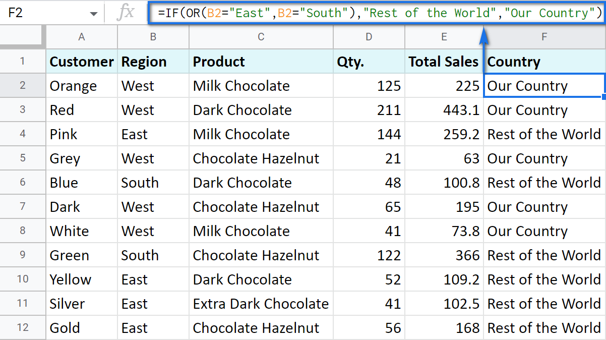
To apply this knowledge to the table with sales, mention all the regions that belong to the sales abroad, and the other sales will automatically become local:
=IF(OR(B2="East",B2="South"),"Rest of the World","Our Country")
Google Sheets IF AND
The AND function is just as simple. The only difference is that it checks if all listed logical expressions are true:
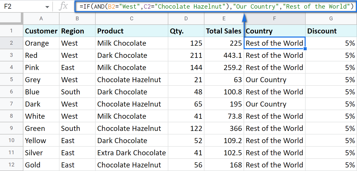
E.g. you need to narrow the search to your town and you know that it is currently buying only hazelnuts. So there are two conditions to consider: region – "West" and product – "Chocolate Hazelnut":
=IF(AND(B2="West",C2="Chocolate Hazelnut"),"Our Country","Rest of the World")
Nested IF formula vs. IFS function for Google Sheets
You can also use the IF function itself as an argument for the bigger IF function.
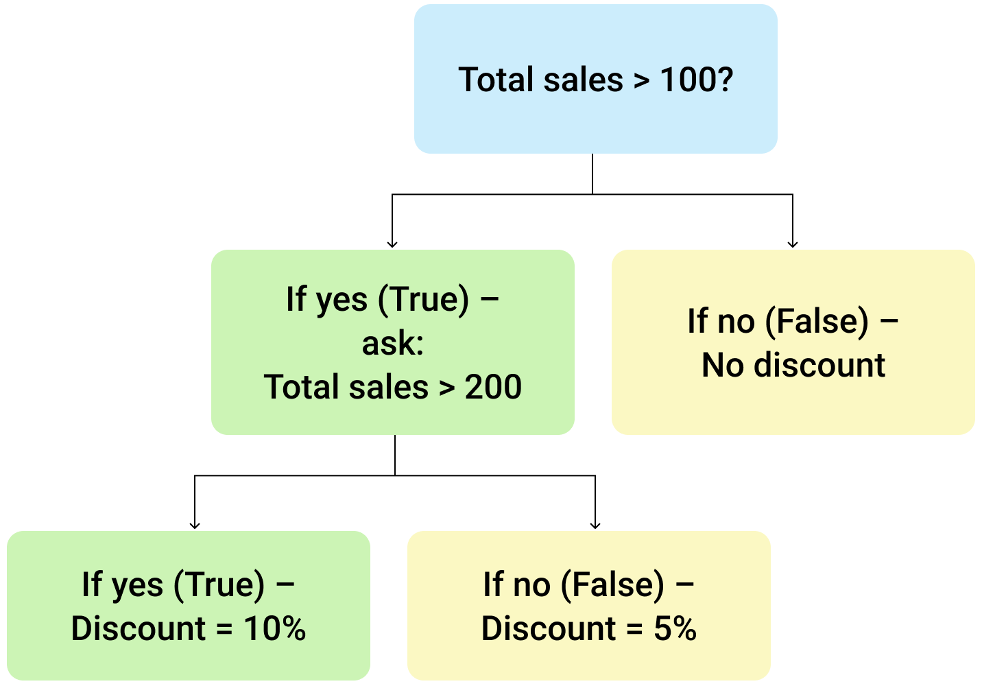
Let's assume that you have set stricter discount conditions for your clients. If the total purchase is more than 200 units, they get a 10% discount; if the total purchase is between 100 and 199, the discount is 5%. If the total purchase is lower than 100, there is no discount whatsoever.
The following formula shows how the function will look in the cell G2:
=IF(E2>200,E2*0.1,IF(E2>100,E2*0.05,0))
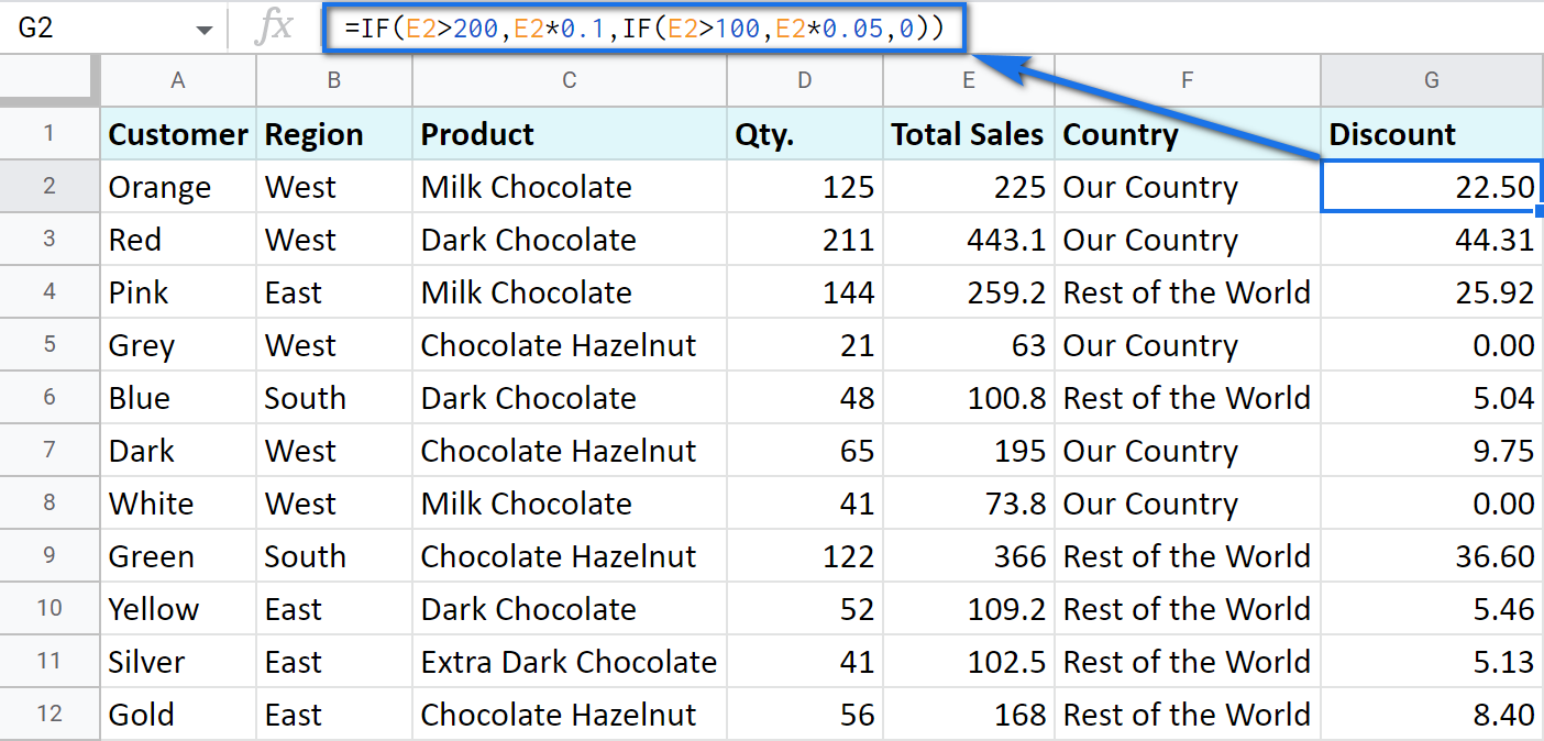
Note that it is another IF function that is used as the second argument. In such cases, the decision tree is as follows:
Let's make it even more fun and complicate the task. Imagine that you're offering the discounted price to the one region only - "East".
To do that correctly, add the logical expression "AND" to our function. The formula will then look the following way:
=IF(AND(B2="East",E2>200),E2*0.1,IF(AND(B2="East",E2>100),E2*0.05,0))
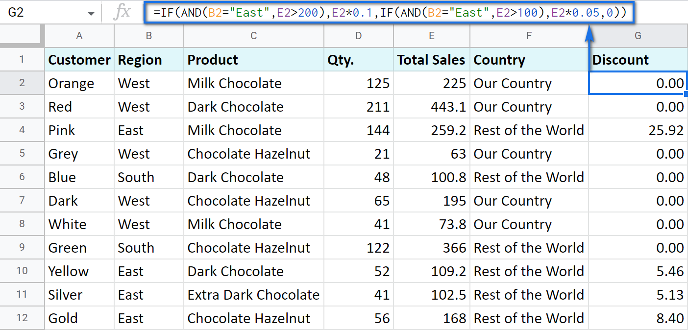
As you can see, the number of discounts has reduced greatly while their amount remains intact.
There's also an easier way to write the above thanks to the IFS function:
- condition1 – (required) is the logical expression you want to test.
- value1 – (required) is the value to return if the condition1 is true.
- and then you just list conditions with their values to return if they are true.
Here's how the above formula will look with IFS:
=IFS(AND(B2="East",E2>200),E2*0.1,AND(B2="East",E2>100),E2*0.05)
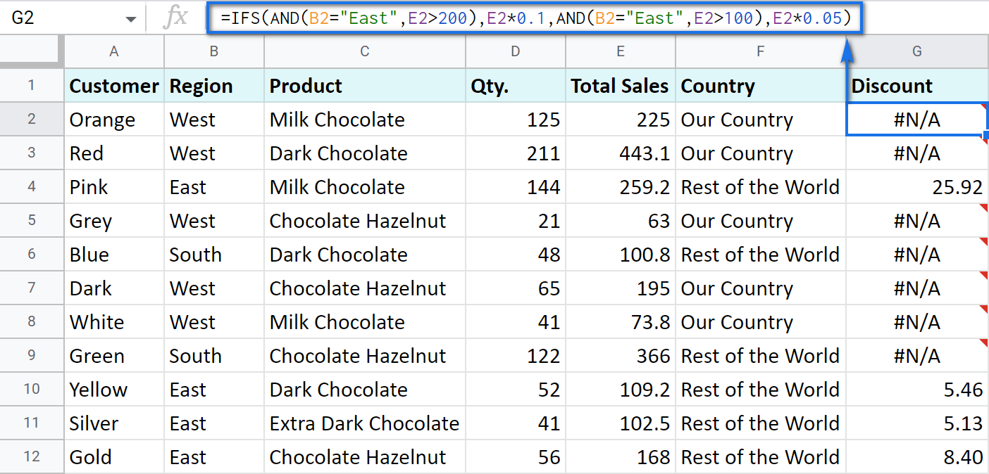
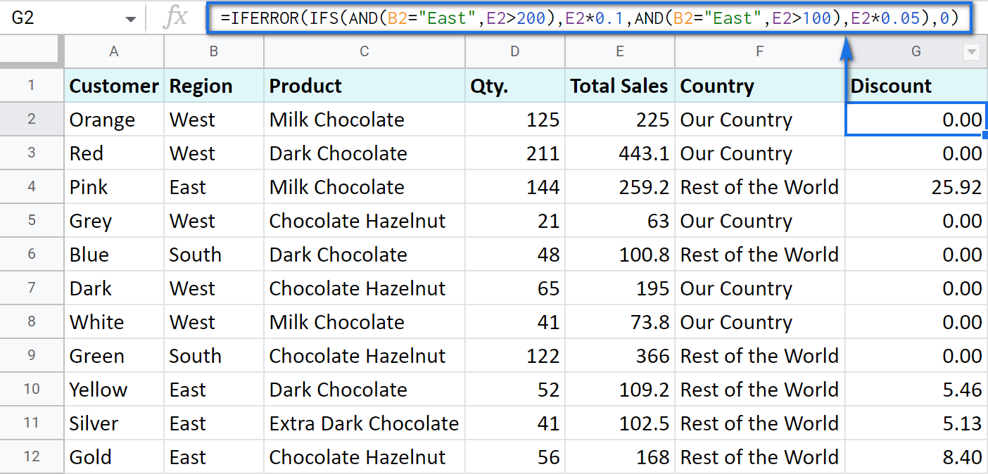
Tip. If there's no true condition, the formula will return the #N/A error. To avoid that, wrap your formula with IFERROR:
=IFERROR(IFS(AND(B2="East",E2>200),E2*0.1,AND(B2="East",E2>100),E2*0.05),0)
SWITCH as an alternative to multiple IFs
There's one more function you may want to consider instead of the nested IF: Google Sheets SWITCH.
It checks if your expression corresponds to a list of cases, one by one. When it does, the function returns a corresponding value.
- expression is any cell reference, or a range of cells, or even an actual math expression, or even a text that you'd like to equal to your cases (or test against the criteria). Required.
- case1 is your first criteria to check the expression against. Required.
- value1 is a record to return if the case1 criterion is the same as your expression. Required.
- case2, value2 repeat as many times as criteria you have to check and values to return. Optional.
- default is also completely optional. Use it to see a specific record if none of the cases is met. I'd recommend using it every time to avoid errors when your expression doesn't meet matches among all the cases.
Here are a couple of examples.
To test your cells against a text, use ranges as an expression:
=ARRAYFORMULA(SWITCH(B2:B69,"West","Our Country","Rest of the World"))
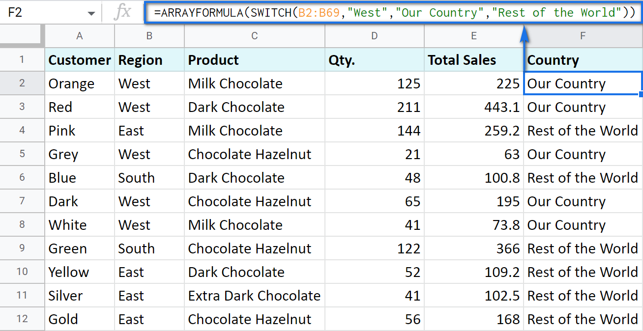
In this formula, SWITCH checks what record is in every cell in column B. If it's West, the formula says Our Country, otherwise, Rest of the World. ArrayFormula makes it possible to process the entire column at once.
To work with calculations, it's better to use a boolean expression:
=SWITCH(TRUE,$E2>200,$E2*0.1,AND($E2<200,$E2>100),$E2*0.05,0)
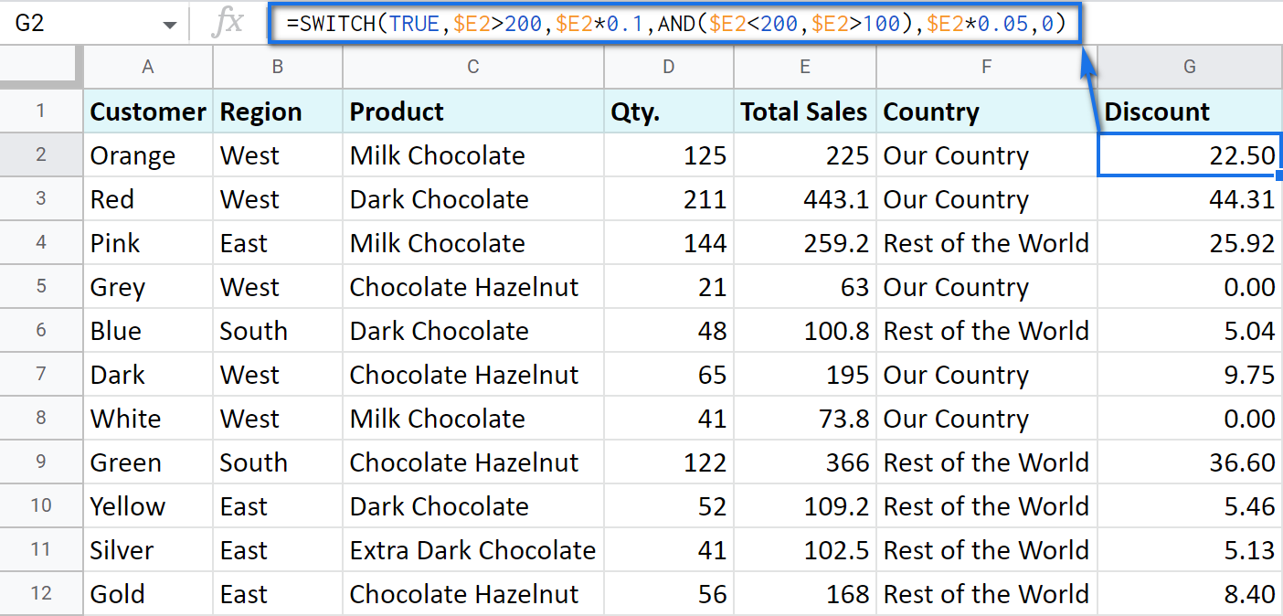
Here SWITCH checks if the result of the equation is TRUE or FALSE. When it's TRUE (like if E2 is really greater than 200), I get a corresponding result. If none of the cases in the list is TRUE (meaning they are FALSE), the formula simply returns 0.
Note. SWITCH doesn't know how to calculate the entire range at once, so no ARRAYFORMULA in this case.
IF statements based on a count
One of the questions we get asked a lot is how to create the IF formula that will return whatever you need if the column contains or doesn't contain a certain record.
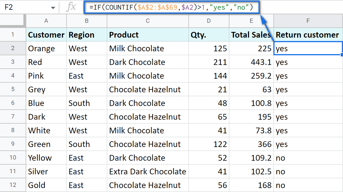
For example, check if a customer's name appears more than once in a list (column A) and put the corresponding word (yes/no) into a cell.
A solution is simpler than you may think. You need to introduce the COUNTIF function to your IF:
=IF(COUNTIF($A$2:$A$69,$A2)>1,"yes","no")
Make Google Sheets build IF formulas for you – IF Formula Builder add-on
If you're tired of keeping track of all those extra characters and proper syntax in formulas, there's another solution available.
IF Formula Builder add-on for Google Sheets offers a visual way of creating IF statements. The tool will handle syntax, extra functions and all required characters for you.
All you need to do is:
- fill blanks with your records one by one. No special treatment for dates, time, etc. Enter them as you always do and the add-on will recognize the data type.
- select required comparison operators from the suggested drop-down lists.
- if needed, add multiple logical expressions in a click: IF OR, IF AND, ELSE IF, THEN IF.
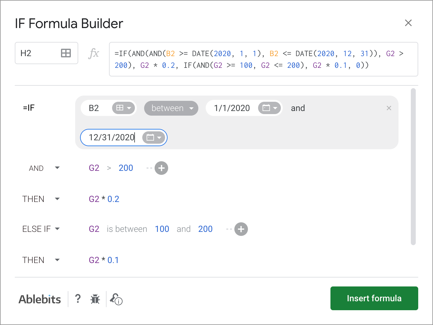
As you can see, each logical expression takes its own line. The same goes for true/false outcomes. This reduces the number of possible confusion over the formula drastically.
As you fill everything out, the formula for use will grow in the preview area at the top of the window. To its left, you can select a cell in your sheet where you'd like to have the formula.
When you're ready, paste the formula into the cell of interest by clicking the Insert formula button at the bottom.
Please visit the online tutorial for IF Formula Builder to see all options described in detail.
I hope that there's no room for any doubt now that the IF function, though a very simple one at first glance, opens the door to many options for data processing in Google Sheets. But if you still have questions, feel free to ask them in the comments section down below – we'll be happy to help!
 by
by
590 comments
DROP BOX = MALAYSIA,SINGAPORE,FILIPINE
how.
select malaysia = 17% /
select singapore = 16%
please help
Hello Emma,
Please look through these instructions to build the formula correctly.
Hi, can you help me how to make a formula that based on the covered period time it will call the window:
1st window
4-8PM
2nd window
8-12MN
3rd window
12MN-4AM
4th window
4-8AM
5th window
08-12NN
6th window
12-4PM
Thanks.
Hi Russle,
If I understand your task correctly, you should use the Apps script to call for windows. We're always ready to help you, but we do not cover the programming area (script-related questions). You may try to find a solution here – an overview of Google Apps Script with a lot of helpful content and links:
https://developers.google.com/apps-script/overview
HELLO,
PLEASE HELP
IF A CELL CONTAINS 50% OR ABOVE THEN CLASS 1 OR BELOW 50% THEN ECE.
FORMULA IN CELL A2
CONDITION IN CELL A1
Hello Neha,
here you go:
=IF(A1>=50,"CLASS 1","ECE")
Hello,
Can you let me know where i am going wrong. it says i have only imputed 1 argument.
=IF(OR(IMPORTRANGE("https://docs.google.com/spreadsheets/d/1EjfESGzrXaeh6oaWrZWMGOuCEzgdgFQpO6pzEMZxpJc/edit#gid=1328129828&range=J5:J66", "bennys tune sheet.!J5:j66")="YES",(IMPORTRANGE("https://docs.google.com/spreadsheets/d/1EjfESGzrXaeh6oaWrZWMGOuCEzgdgFQpO6pzEMZxpJc/edit#gid=1328129828&range=J5:J66", "bennys tune sheet.!J5:j66")="NO"),"YES", "NO"))
Many thanks in advance, and thank you all for the amazing guide :D
Hello Alex,
There are a couple of excess brackets. Here's a correct formula:
=IF(OR(IMPORTRANGE("https://docs.google.com/spreadsheets/d/1EjfESGzrXaeh6oaWrZWMGOuCEzgdgFQpO6pzEMZxpJc/edit#gid=1328129828&range=J5:J66", "bennys tune sheet.!J5:j66")="YES",IMPORTRANGE("https://docs.google.com/spreadsheets/d/1EjfESGzrXaeh6oaWrZWMGOuCEzgdgFQpO6pzEMZxpJc/edit#gid=1328129828&range=J5:J66", "bennys tune sheet.!J5:j66")="NO"),"YES","NO")
BTW, have you seen our IF Formula Builder from the last part of the article? It worries about the correct syntax for you so I'd suggest you check it out :)
Hi! and thanks for a great article, very helpful. I am hoping you can help me with what is possibly a very basic function - I want to create a signal between the change of two numbers. For example, if on Tuesday the number in cell A1 is 10 and on Wednesday the number in cell A2 is 5, I would like a trigger cell to tell me that there has been 50% change from one day to the next.
Can you please help me with this? Thanks so much!
Patrick
Hello!
Use this formula and set the percentage format in the cell:
=(A2-A1)/A1
Hi I am looking at using the IFs function however, I want it to return a cell from another sheet or be able to return a true statement that has skipped lines if you know what I mean IE
in A1 = Apples and I want my True statement to appear as:
B1 Red
Apple
Sauce
Rocks
instead of Red Apple Sauce Rocks?
Hi Sarah,
you can either press Alt+Enter when you type the formula to wrap the words,
or insert line breaks using a true statement like this: "Red"&CHAR(10)&"Apple"&CHAR(10)&"Sause"&CHAR(10)&"Rocks"
Related text need to display in 1st table from the 2nd table, If we write a remarks in the 2nd table following and related text in the 1st table -- can any one write the if formula for this
Hello Suresh,
I'm afraid there's not enough info to provide you with a formula. Please describe your task in detail so we could help.
DOH logic flow
5 & 7 & 10 day- Priority P4
How can I run this logic in google sheet? Please help on urgent note.
Hello Sanjeev,
You need to include AND function into your IF formula. You will find examples in this part of the article.
I am using a simple IF statement to populate a numerical value. I then use that value for another calculation and a SUM at the bottom the section.
It's not reading the number as a number in the SUM function, but it is in the other cell.
I've also tired saving and opening in Excel.
I'd so appreciate suggestions, it's making me crazy LOL.
Analyze request 2 1
Is the data in Personas? Yes =IF(H4 = "yes", "2", "8") =I4/3
Is the destination in Self Service? No =IF(H5 = "yes", "0", "8") =I5/3
Requirements LOE Estimate =SUM(I3:I5) =SUM(J3:J5)
Analyze request 2 1
Is the data in Personas? Yes 2 1
Is the destination in Self Service? No 8 3
Requirements LOE Estimate 2 4
Hello Rebecca,
When you put numbers in the IF formula in double quotes, the formula returns them as text because this is how text is written in formulas. To have numbers as numbers, remove those double quotes from around your numerics, like this:
=IF(H4="yes", 2, 8)
how would i do an if statement like "if there is nothing in the cell above, move everything to cell above?" Is it possible to do that?
Hello Eletron,
I'm afraid you won't be able to do that with formulas. You see, formulas return results into cells where they are entered. Also, you can't enter the formula into a cell and check that cell for any condition at the same time. In other words, if you enter the formula to B2 and check if B1 is empty, the result will be returned to B2.
What's more, you cannot cut-paste data using formulas, only copy-paste it. So any data joined from other cells in B2 will also remain in all other cells.
oh ok
Is there a function that would be true if the cell of interest contains any of the words in a specified column? I was going to use an IFS statement to tag rows based on what they contain.
Hello Danielle,
If I understand you correctly, you can use either nested IF or IFS. Both will do just fine. Please read this point of the blog post for more details and formula examples.
I'm trying to have a cell automatically round up no matter if the value is less than .5 or not. I need the value to round up always. So for instance if the value is 2.35, I need it to round up to 3.
Thank you!
Hello Amanda,
Google Sheets has the ROUND function, it will help you. Please look for the instructions on this Docs Editors Help page.
So I'm trying to use a pretty basic IF OR formula in Google Sheets: =IF(OR(I299),"I2","").
The trick is that for my value if true, I want to use a cell reference, not just a static value / word. When I use just the IF statement without OR, it accepts I2 as a cell reference, but when I make it an IF OR it no longer recognized my "value if true" as a cell reference.
Is there anyway to adjust that?
Hello Natalie,
If you want I2 to be treated as a cell reference, you should omit double-quotes. Double-quotes make values text strings.
Also, OR requires some condition, not just a cell reference, and is usually used to list several conditions to see if at least one of them is true. Hence, the correct formula for you should look like this:
=IF(I299=SOMETHING,I2,"")
If that doesn't really work for you, please describe your task in detail and I'll help with the whole formula.
if the two column cells are red in colour then write 0.5 in another column how to write a formula can you please tell any one
Hello Sethu,
There are no standard formulas that would check cell colors. We have a special tool for that: Function by color. You can use it to count colored cells. However, it can’t return the value you need based on colors. You will need to build the simplest IF formula afterwards to return 0.5 if our add-on returns 2.
Hi everyone,
I've read thru many comments but still not understanding exactly how to approach my specific calculation need.
My need is specific to the Canadian Recovery Benefit, which has a cap of 18K for my situation. I am allowed to make up to 38K in salary/profit without penalty or obligation to reimburse any portion of the 18K. But for every dollar made over 38K that I make (with the exlusion of the 18K govt benefit) I would need to reimburse half of the benefit received (0.50) until I reach the threshold where I am obligated to reimburse all of it (which if my calc is correct, is 74K total salary).
ie. If I make 38K or less, and also receive the 18K govt benefit, I am not obligated to reimburse any of the benefit. I am naturally obligated to pay the income tax on the 56K total.
If I make 48K (exluding the govt benefit), I am obligated to reimburse 5K of the 18K govt benefit received. 0.50 cents per every dollar of the 10K I am over the limit.
If I make 74K (excluding the govt benefit), I am obligated to reimburse the full 18K govt benefit. (74K being the threshold of 38K, plus 2X the 18K maximum benefit)...
I'm trying to generate a sheet in which I can enter the amount of money I have made to date into one cell, and have the sheet tell me 1) If I am over the limit - this calc is easy, and, 2) tell me how much I need to reimburse in the even that I make of over the 38K.
I am assuing this is not that hard, but the formulas for it are above me.
Here's as far as I got:
=IF(I41=">$38,000.00","No Pay", "Pay") this would simply alert me if I had crossed the threshold and needed to pay. Its not very elegant, but for the first part seems to work.
But what formula (or addition to the original) would tell me how much of cell I41 would be payable if it crossed the 38K...? Iaking into account the .50 of every 1.00 more made... I hope this makese sense.
Any help or tips to making this work are greatly appreciated. Thank you!
Bob
(a rudimentary preview of the issue)...
https://www.dropbox.com/s/zzbqe32xac09mcb/Screen%20Shot%202021-03-11%20at%209.59.16%20PM.png?dl=0
Hi Bob,
Thank you for the detailed description and the screenshot. If I understand your task correctly, the following formula should do the trick:
=IF(I41<=38000,"No Pay",IF(AND(I41>38000,I41<74000),(I41-38000)/2,18000))
Hi
I am trying to populate a yearly expense dashboard I created. I have sheets for every month. In column B (expense category "Grocery") and column D ($ amount)
I am trying to add all values in Column D ($ amount) that have "Grocery "in column B to populate a monthly total for groceries on my dashboard.
I am tired of sorting the column by category and redoing the formula to calculate totals every few week.
Is this possible?
Hi Natan,
I'm sorry I'm afraid I need more details on your task to be able to suggest anything.
Please create a small sample spreadsheet with (1) a couple of sheets with the example data and (2) with a sheet showing the result you want to get. Then share this file with us: support@apps4gs.com. I kindly ask you to shorten the tables to 10-20 rows.
Note. We keep that Google account for file sharing only, please do not email there. Once you share the file, just confirm by replying to this comment.
I'll look into it and see what may help.
Hi I have sent this.
Hi Natan,
Thank you for sharing a sample. You need to use the SUMIF function for the task. I entered the correct formulas to the first 3 columns on the Dashboard sheet so you could see what to do. If you need more details on the SUMIF function, we have a cool blog post about it, feel free to look through :)
I am working with schedules, for Example: 0300-1100,1100-1900,1900-0300 three different shifts, How can I make all 0300-1100 scheduled employee names appear in a group?
Thank you
Hello Jake,
Please create a small sample spreadsheet with 2 sheets: (1) example data, (2) the result you want to get, and share it with us: support@apps4gs.com. I kindly ask you to shorten the tables to 10-20 rows.
Note. We keep that Google account for file sharing only, please do not email there. Once you share the file, just confirm by replying to this comment.
I'll look into it and try to come up with a solution.
Hi Natalia,
I just shared the spreadsheet to that email. Thank you.
Hi Jake,
I've got the file, thank you.
Please look at B16, B19, D16 and D19. I used QUERY to return the required records. You just need to create similar formulas for other days.
The same can be done (with and without formulas) with our Multiple VLOOKUP Matches add-on.
Also, B3:I12 contained some excess spaces that prevented from getting the correct results. I trimmed them with our Remove spaces tool.
Hope this helps!
Want to set True if cell contains a specific word. How to do that?
for ex: Let's say cell F4="Rest of the world". Then, if "Rest" contains in the cell F4, set True, else False.
Hello Pritam,
Try this formula:
=IF(ISNUMBER(SEARCH("rest",A2)),TRUE,FALSE)
I am trying to create a IF formula where IF cell P2 = Y then "Need to be invoiced" is entered into Q2, however, if R2 has a date inputted into it, Q2 will have "Invoiced" into it. I am having trouble as I get one or the other to work but not together.
Hello Stacy,
Try this formula:
=IF(ISDATE(R2),"Invoiced",IF(P2="Y","Need to be invoiced",""))
That formula worked with the exception when P2 is yes but there is no date in R2, the Need to be invoiced did not populate. do I need either an OR or And function in there?
Nevermind - I figured it out! P2 uses the word "Yes" not just a "Y" as soon as I fixed that it worked.
Thank you for your help!
Thank you for letting me know, Stacy.
Good to know you found the solution!
Hi, I am looking for a formula to help with our staff holiday tracking sheet. We have a new policy where holiday entitlement run from Birthday to birthday or each staff (we used to run the from 01/01 to 31/12) As it is our first year doing this it will have run from 01/01 until their birthday this year and then start again. I need a formula that will: one, pull through the start date of the holiday year and the end date and two, change date after the birthday has passed this year. I also then need one that will calculate how man holiday days are accrued between the start and end date of the holiday year.
E2 - Staff name
E3 - Holiday year start date (Need formula for this)
E4 - Holiday year end date (Need formula for this)
E5 - Holiday entitlement (need formula)
A separate page will have all names and birthdays.
Sheet name is Bdays - A1 has the bday date in (12/02/2021)
Any help would be much appreciated. Im unsure if i need a Vlookup, or IF or maybe both?
Hi Michaela,
Do you intend to use a drop-down list of names in E2 and want other cells to change accordingly or you'd prefer having each staff member's info displayed at the same time?
For me to understand your task better, please share a small sample spreadsheet with us (support@apps4gs.com) with an example of your data and the result you expect to get. I kindly ask you to shorten the tables to 10-20 rows.
Note. We keep that Google account for file sharing only, please do not email there. Once you share the file, just confirm by replying here.
I'll look into it and try to come up with a solution.
I created an order form for my craft shows and want the prices to populate when i select each item. I figure its an If:Then type of situation but Its been a long time since I've worked on things like this and could use some guidance
Column B= Item Description
Column D= Price
I made a drop down list for column B to show all the items I currently have in stock. I also have a drop down list in Column D and can manually click on each price. I would love to figure out the proper way to bypass this.
Example: Items- lollipop and chocolate are $1 each. bubbles, reindeer food, lip balm, and hand sanitizer are $3 each.
Do I need to say something like If B=lollipop or chocolate then D=$1???
Hello Jessica,
Yes, you will need to use the OR logic in your nested IF, like this:
=IF(OR(B2="lollipop",B2="chocolate"),1,IF(OR(B2="bubbles",B2="reindeer food",B2="lip balm",B2="sanitizer"),3,""))
The following parts of the blog post above will help:
How do i make the cell that has the formula in it blank until it populates? at the moment it has FALSE until the other cell is written in ?
Hello Tania,
Use a pair of double quotes as an argument to indicate a blank cell, like this:
=IF(A2="West","Yes","")
I would like to total the prices (Column D) of rows assigned in Column G. I have Data Validation to make a dropdown of values "1-4" (column G). I want to sum the values of all group 1 column D's, all group 2 column D's, etc to another cell.
Hello Dave,
To total numbers based on records in other cells, you need to use the SUMIF function. We have a nice tutorial about it, please take a look:
SUMIF in Google Sheets
Could you please help me with a formula,
IF the cell is EE then the number is 3, if the cell is ME then the number is 2, if the cell is NW , then the number is 1.
Hello Rogelio,
Assuming your cell is A2, here's a formula you can use:
=IF(A2="EE",3,IF(A2="ME",2,IF(A2="NW",1,"")))
My business focuses on retail, contractor, wholesale sales, but also includes stock. We do batch ordering and a majority of what we order is already pre purchased. I am trying to separate in one column a letter for each: R, C, W are what we are using as our definers. We want a count from each grouping, and also a percentage. Please help....
Hello JB,
If I understand your task right, you may find the following blog posts helpful:
Split text to columns in Google Sheets
Google Spreadsheet COUNTIF
Google Sheets percentage formulas
If I want to past a formula into consecutive vertical cells but want to keep ONE of the sections of the formula the same, is this possible? When I paste it, the L30 goes to L31 then to L32, etc., and the D1 goes to D2 to D3, etc. I'm wanting the L to stay at 30 and the rest to move with each line.
e.g., If I paste =IF(L30>=12.5,D1*25%,D1*20%) in A1, and =IF(L31>=12.5,D2*25%,D2*20%) in A2, and =IF(L32>=12.5,D3*25%,D3*20%), etc., etc.
Hello again, Kevin,
Yes, it's possible: proper cell references will do that for you. Please have a look: types of cell references.
That is great! Thank you!
My pleasure, Kevin :)
Hello Natalia, I'm need to have multiple IFS and am having trouble with the formula. I need a cell to populate a dollar amount based on a percentage range in another cell. If the percentage is between 11 - 11.99 = $125, 12 - 12.99 = $250, 13 - 13.99 = $375, 14 - 14.99 = $500, 15 or more = $750. How can I write this formula?
Thanks
Hello Kevin,
When it comes to IFS, you simply need to alternate your criteria with its result. The example is illustrated here.
Assuming the percentage starts in A2, here's how the formula should look like:
=IFS(AND(A2>=11,A2<=11.99),125,AND(A2>=12,A2<=12.99),250,AND...,etc,etc)
PERFECT! Thank you!!!
I'm trying to black out cells if the cell prior has N/A from a drop down list. This would also need applied to the entire column.
Thank you in advance!
Hi Kim,
I'm sorry but your task is not clear.
For us to be able to help you, please share a small sample spreadsheet with us (support@apps4gs.com) and include two tabs there: 1 - your source data, 2 - the result you need to get.
Note. We keep that Google account for file sharing only, please do not email there. Once you share the file, just confirm by replying here. Thank you.
Maybe an Example sheet is easier:
https://docs.google.com/spreadsheets/d/1CmkI8pyqC0oHKVXH0JIRL_yb9BbasbrIbAvy2NO-hio/edit?usp=sharing
Hello William,
Though your formula works on my side, I'd adjusted it a bit:
=ARRAYFORMULA(IF($J4:$J="name",$H4:$H*0.85,IF($J4:$J="","",0)))
ArrayFormula auto-populates the entire column with the formula while the second IF returns an empty cell for those rows where column H is not yet filled with data.
I tried to look into your file, but I can't access it. If you still need my assistance with the formula, please share an editable copy of your spreadsheet with us directly: press the Share button at the upper right corner of your spreadsheet and enter support@apps4gs.com.
Note. We keep that Google account for file sharing only and don't monitor its Inbox. Please do not email there. Once you share the file, just confirm by replying here. Thank you.
I'm trying to make a formula but I can't seem to find the answer to what I try to achieve.
What i'm trying is to automatically subtract a percentage on an array when the cell next to it contains a name.
=IFERROR(IF($J4:$J = "name", $H4:$H*0.85, $H4:$H*0))
So if a cell in array J contains a "name, the cell left of where the name is substracts 15% That my formula is wrong, is for sure! But where? Thank you in advanced.
Hi,
figured it out finally!
=IF(O$5>=$H6,if(O$5<=$I6,$D6,""),"")
Patience and time solves everything!
Thank you for the follow-up, Scott,
Good to know you figured the solution out :)
Hi,
This is for a construction project...looking to put how many people will be on a job for each day. Using Google sheets....
I have the dates in the main cell as follows:
P5 is the date in question 5/26/2020
H6 is the start date 5/26/2020
I6 is the end date of the project. 11/9/2020
once i run this formula i can make all cells (for this job) a specific color Perfect, and starts on 5/26/2020 stops on 11/9/2020.... :)
=AND(O$5>=$H6,O$5=$H6,P$5<=$I6,D6*1,"")
this does give a blank for the false but how do i get the true statement to read the D6 cell?
Is there a way to get this number into each cell for the job by not typing it in. Seem so simple yet i am at a loss.
any help would greatly appreciated
Thank you
Hi,
I was wondering if I could receive some help with a formula. I'm trying to figure out how to create a scenario where I can view the commission rate (it differs by company) by company?
It would be such that column B (where the companies are) would dictate the percentage of commission that's taken, and the percentage is taken from the sum of columns K-M. I want to create a commissions column in column N, and would like for the formula to run the length of the column.
The % taken is such that Company B has 33% taken, Company IT, S-Corp, and AA has 28% taken, and every other company has 25% taken. I've linked the sheet below for easier viewing:
https://drive.google.com/file/d/1SZ3U1SXiorYnsTt9566ymPWQDX734CY_/view?usp=sharing
Thank you!
Hi Amanda,
Thank you for the description and the file.
To calculate the commission rate by company, use this formula in B7 and copy it down the column:
=IF(B7="","",IF(B7="B",33%,IF(OR(B7="IT",B7="S-Corp",B7="AA"),28%,25%)))
To deduct the percentage from the total of columns K-M at the same time, here's another formula:
=IF(B7="","",IF(B7="B",SUM(K7:M7)-33%,IF(OR(B7="IT",B7="S-Corp",B7="AA"),SUM(K7:M7)-28%,SUM(K7:M7)-25%)))
Hello,
Can you please help?
I would like a formula to do the following. I have three columns. Column 1 are a list of dates, Column 2 is also a list of dates, Column 3 is a list of number. I want a sum of column 3 for only the following cells. Cell 1 has a value and Cell 2 does not have a Value.
Hello Pierce,
You should use the SUMIFS function to do that, it is described in this blog post. Please pay closer attention to a part explaining how to sum one column if cells in other columns are (non)-blanks.
I've used an IF statement to populate a column with a '1' for a true value and a '0' for a false value. In another cell, I want to sum all of the '1' values but the sum formula isn't picking them up. Is it possible to sum up all of the 1 values returned from all of my IF statements?
Hello Harry,
Can you please share the exact formula you're using to sum those numbers returned by IF?
Hi Natalia,
I managed to resolve myself thanks. The problem was I has quotation marks around the true and false values which was stopping them displaying as values that could be summed.
My original statement was =IF("B3=Test","1","0")
And changing it to =IF("B3=Test",1,0) has fixed it.
Hi Harry,
Thank you for the update. Good to know you managed to fix the formula!
Double quotes are used for text strings. When used with numbers, they turn numerics into the text and prevent them from being calculated.
Hi
I am trying to pick shipments from a list whch has columns with several information. I try to fix a correct formula which gives me the result 1 or 0, or True or False or a colour or whatsoever.
Lets say I want the in Cloumn T see the result if either one of the conditions are fullfilled. Aka if one of the conditions is fullfilled should the result be 1/True/Green cell, etc.
First condition: IF C3<=3,99 and D3<=999
2nd condition: IF G3="Yes" and E3<=3
3rd condition: IF C3=6 and D36 and D3>1000 and D3<2500
I do not know what I am doing wrong, but I don't get it together, and with only 2 conditions (which are probably wrong) I get 1 as a result for a row with "yes" in cloumn G, whereas if the data in the column is "no", but it fullfills i.e. the first condition, the result is instead of 1, true? Appreciate your help so much. Thank you!
Hi
I forgot the conditions in the 2nd condition
which is if G3 s "yes" and E3<=3 is kind of missing the part, that if E3=1 should D3<=800, but in case E3=2 should D3<=1600 or in case E3<=3 so should D3<=2400
how is it possible to combine all the conditions in a formula?
Sorry for the unconvinience.
Looking forward to your reply
Kindest regards
Hi Fatos,
I'm sorry but it's hard to get a clear understanding of what you're trying to achieve.
For me to be able to advise you anything, please consider sharing a small example spreadsheet with us (support@apps4gs.com) with 2 sheets: a copy of your source data and the result you expect to get. Please include the formula that doesn't work as well and shorten the tables to 10-20 rows.
Note. We keep that account for file sharing only and don't monitor its Inbox. Please do not email there. Once you share the file, just confirm by replying here.
In the meantime, please look through the last part of the blog post more closely. It describes how to enter multiple conditions to your formula.
Hi Natalia
Thank you sooo much, I will send you an exempel
Kind regards
Hello
I've shared the file now
thanks again!
Hello Fatos,
I'm sorry, I can see no files shared by you. Please follow these steps to share the file correctly:
The file will then appear in the Shared section of our Drive. For more details on sharing the files, please turn to this help page. Thank you.
Hi,
so sorry, I'll try to send it again. Sorry for the unconvenience... In the meantime did I manage to find I formula which appears to work. But I am not sure if that is the best way to do it. I'll try to send it now
Thanks a lot & sorry again
Hi there
1 - I've shared as requested a simple version of the file. hope it worked this time
2- does anybody know how I can create an automated list of tabs/sheets in the same worksheet. Its a schoolproject; a (daily) spreadsheet with over 70 tabs/sheets and we need to have a summary-tab (we need to "analyze" data for a period of 120 days, and have no knowledge or info on coding etc)
All kind of help is greatly appreciated
Thank you!
Hi Fatos,
Thank you, I've got the file. I'll look into it as soon as possible.
As for your second question, we have an article describing different ways of combining data from multiple sheets, make sure to check it out.
Hi,
Thank you again.
Re my second question; I need to get a list of the tabs in another (summary tab) tab of the same spreadsheet. Like an index, which I want to use to create a table and "extract and summarize" information, so the names of these tabs are going to be the rows in this table. I was not able to find the funtion to use for this
Kindest regards
Hi Fatos,
I looked into your file. I created an additional column Q, named it Ablebits, pasted the formula there, and copied it down the column. Here it is:
=IFERROR(IFS(AND(M2<=2,4;K2<1000);1;AND(AND(M2>2,99;M2<=6);K2<=50);2;AND(M2="pall";AND(N2>0;N2<=3);K2/N2<=800);3);0)
The formula returns 0 instead of the error when there's no match to any of your conditions. Also, the column cells turned green due to the existing conditional formatting, but I'm not going mess with that. Please adjust your conditional formatting accordingly.:) Hope the formula solves the first task for you.
As for the second one, I appreciate the additional info. But I'm afraid there's no easy way to avoid entering each sheet name manually. I'd advise you to search for a solution here - an overview of Google Apps Script with a lot of helpful content and links: https://developers.google.com/apps-script/overview
I wish I could help you better.
Thank you for all your help !
Have a great day...
Fatos
I have a sheet where data copies from a master tab to a slave where I want some information removed or hidden as it will be shared outside our business. What I would like to achieve is IF it reads (in this case) 4S then the information shows on that second tab, and IF it reads anything else, for example CL, RN or EC then it does not automatically show on the second tab. This is all very new to me so would appreciate if you could advise how I go about this...
Hello Bronwyn,
If I get your task correctly, you should pull data using the QUERY function since you can add conditions for pulling there. I explained how it works in this blog post.
I am trying to utilize Google Sheets to take a list of email addresses and see if it has ever been seen before.
Emails are listed in Colum C and my string is:
=IF(C2="C2;C1000","YES","NO") however it is returning NO no matter if it has been seen before.
Hello Hayden,
a simple IF is not enough here, I'm afraid. You should incorporate the COUNTIF function to your formula:
=IF(COUNTIF(C2:C1000,C2)>1,"YES","NO")
Hi, I need help correcting this formula which refers to a VLOOKUP before an IF command with an "and" condition:
=IF(VLOOKUP(B69,$B$25:$C$43,2,FALSE)10000,C2560000,1800)))
Hi Therese,
I believe, you just miss the comparison before 10000. If you're looking if the match equals to 10000, it should be:
VLOOKUP(B69,$B$25:$C$43,2,FALSE) = 10000
Replace the equal sign with whatever comparison character suits your case.
Also, there are two excess closing brackets at the very end of the formula.
Most helpful and clear explanation on the internet. I seem to have encountered a problem. The cell I'm referencing has drop-down selector. The value of that cell from my view is whatever value has been selected. But the true statement never returns as true but only as false. =IF(E7="Business Analyst", "BA", "Nope") that only ever returns "Nope" despite that Business Analyst is selected and visible in the cell. Will this just not work or is there some other magic?
Hello Christopher,
Thank you for your lovely feedback!
Please make sure the values in your Data validation are written exactly the same as you put them into your IF formula. I mean you should keep the same text case, spacing, etc. If you're still unable to make it work, please consider sharing a small sample spreadsheet with us (support@apps4gs.com) where the problem occurs. I kindly ask you to shorten the tables to 10-20 rows.
Note. We keep that Google account for file sharing only, please do not email there. Once you share the file, just confirm by replying here.
I'll look into it and do my best to help.
Hello, I'm trying to condition a formula to pull info from two columns and then recognize which country it belongs to and from there show one number. So far I'm only able to pull from the first option "US" and if it pulls "CN" shows up as blank.
=ARRAYFORMULA(IF(B5:B50="","",(IF (C5:C50="US",(Items!B2:B50),(IF(C5:C50="CN",(Items!C2:C50),(IF(C5:C50="UK",(Items!D2:D50)))))))))
Hello Andie,
I'm sorry but I'm a bit confused by the formula without seeing the data structure. Would you mind creating a small example of your data and share it with us (support@apps4gs.com)? I kindly ask you to shorten the tables to 10-20 rows. Please include your formula there as well. I'll look into it and see what may be wrong.
Note. That account is for file-sharing only, please do not email there. Once you share the file, just confirm by replying here.
Hello Natalia, thank you for your help
I try to create a google sheet which picks up by name (drop down menu) a multiplication.
example - if cell A2 = x then Cell B2*'Another Sheet'!A2' if cell A2 = y then B2*'Another Sheet'!A3' etc
I have created a short formula with 3 items but I have 100+ items, might be an easier way or simpler? Would be a lengthy formula with a few brackets at the end :) :)
My formula
=IF(A2="x",B2*'Base Sheet'!B2,IF(A2="y",B2*'Base Sheet'!B3,IF(A2="z",B2*'Base Sheet'!B4)))
Thanks in advance
Hello,
Try using IFS instead:
=IFS(A2="x",B2*'Base Sheet'!B2,A2="y",B2*'Base Sheet'!B3,A2="z",B2*'Base Sheet'!B4,...,...)
You will still have to list every condition and its outcome, but no nested IF is required.
Alternatively, you could try building scripts, but we don't help with that. You may try to find a solution here - an overview of Google Apps Script with a lot of helpful content and links:
https://developers.google.com/apps-script/overview
Hope it'll help.
Hi.
How do I work out a formula if I want to charge 50p for every unit after 50 (the first 50 are free)?
Thank you
Hi Mark,
For me to be able to help you, please describe how your data is arranged. Thank you.
How would I nest more than three if statements in this formula?
=if (h2 = 3560,44190),if(3570,44290),if(3580,43390),if(3590,43490),if(3600,43590),if(3610,43690),if(3620,43790),if(3630,43890),if(3640,43990),if(3650,44090),if(3660,44190),if(3670,44290),if(3680,44390),if(3690,44490))
super simple replacement here but it errors after 3. not sure if I should be using a different method here.
Hello Joe,
Here's how the correct syntaxis should look:
=IF(H2=3560,44190,IF(H2=3570,44290,IF(H2=3580,43390,IF(...,IF(...)))))
Or you can use the IFS function instead:
=IFS(H2=3560,44190,H2=3570,44290,H2=3580,43390,...)
Hello again Natalia,
I have another formula question that is similar to what you helped me with last time. I am sharing the sheet with you now.
What I am needing: I need a count of 1 or .5 next to "TOTAL =" depending on if their is a "SPLIT WITH" or not. If there is a persons name in the "SPLIT WITH" column then it needs to count ".5" and "1" if not.
Thanks
Hello Kevin,
Thank you for getting back in touch!
I've got your file. I'll look into it and reply as soon as possible. Thank you for understanding.
Kevin,
The formula is actually the same as before. You just need to change the ranges and remove one excess condition from the previous formula:
=(COUNTIFS($C$3:$C$52,"<>"&"",$G$3:$G$52,"="&""))+((COUNTIFS($C$3:$C$52,"<>"&"",$G$3:$G$52,"<>"&""))/2)
Copy and paste it to your E1.
Though I'm using COUNTIFS (count based on multiple criteria), you can get to know how COUNTIF works (count by one criterion). The functions are similar and you will understand how these formulas work:
COUNTIF in Google Sheets
Hi,
Let me explain the problem:column A is the asset of Jack & column B is the asset of Pot and column C is difference between A & B.
=IF(A2>B2, "Jack has C2 more asset than PoT ","Pot has B2-A2 more asset than Jack").
Is it correct???
How to add both statement & cell value in same function.
Hi,
An ampersand will help you concatenate strings and cell references:
=IF(A2>B2, "Jack has "&C2&" more asset than PoT","Pot has "&B2-A2&" more asset than Jack")
You will find more info on this and other ways in this blog post: Concatenate in Google Sheets
Hello there
Hi I have a google sheet with guest check in and check out.
my problem is I have the following function for timestamp when a value is entered in column A and gives me current timestamp in column C:
//----
function onEdit(e) {
var ss = SpreadsheetApp.getActiveSheet();
var r = ss.getActiveCell();
//1.Change 'Sheet1' to be matching your sheet name
if (r.getColumn() < 3 && ss.getName()=='Daily Guest Info') { // 2. If Edit is done in any column before Column (I) And sheet name is Sheet1 then:
var celladdress ='C'+ r.getRowIndex()
ss.getRange(celladdress).setValue(new Date()).setNumberFormat("MM/dd/yyyy hh:mm");
}
};
I also have a check box at K5 to be checked at the time of payment so I have a timestamp on J5 with a formula below entered in J5
=if(K5,NOW(),"").
However, if I already have a cheked button on K6 and have a timestamp in J6
whenever I enter a value in A1 all the timestaps stored in J6 change together.
I know this is caused by the formula =if(H5,NOW(),"")
do you have a better formula or function for this issue
Thanks Mack
Hello Mack,
I'm sorry but NOW is the only function that returns a timestamp. It's a volatile function, so it recalculates itself in all cells each time anything is edited in the sheet. Thus, the standard formula is not an option here, I’m afraid. You need to use scripts to solve the task.
Since we don't help with scripts, you may try to find the solution here – an overview of Google Apps Script with a lot of helpful content and links:
https://developers.google.com/apps-script/overview
I wish I could help you better.
hi , my condition is if in priority column value is "high" or "medium" AND in status coloumn value is "open", then "to do" must be printed else "hold" must be printed
how to do this ?
columns are priority(values="high","medium","low"),status(values="completed","open")
Hi Aswin,
I believe this is the formula you're looking for:
=IF(AND(OR($A2="high",$A2="medium"),$B2="open"),"to do","hold")
Maybe someone can figure this out; I'm trying to modify a template I use to keep my checking balance by adding a column that can show me my balance based on what check have cleared, and a balance showing me what my actual balance is, including checks that may not have yet cleared. So, column D is a flag to tell me whether a check has cleared or not that I manually set. If that "x" is not true, or present, I'd like column H to show what is showing in the bank. Any suggestions are appreciated. https://docs.google.com/spreadsheets/d/1CDpexKUMuTcJEgCDXcq1XREFOoyjOsSyfBdISdiStNQ/edit#gid=0
Hello Michael,
I looked into your file and adjusted the formula in column H for you based on how I understood your task. Try putting the below into H5 and then copy the formula down:
=IF(D5="x", $G$4-SUM($E$5:E5)+SUM($F$5:F5), G4)
If that's not really what you're trying to achieve, please describe the task and the desired calculations in more detail.
My question is:
I have two drop downs of salespeoples names (one in column K and column L) and I have another column (AF) that calculates how many times a salespersons name is chosen in column K. I want to know if there is a way that if "James" is used in column K and no name is in column L it produces a numerical count of 1 next to James' name in column AF. But if "James" is in K or L and "Kevin" is in the opposite one, can it produce a .5 for each person in column AF?
Hello Kevin,
For us to get a better understanding of your case, please share a small sample spreadsheet with us (support@apps4gs.com) with 2 sheets: a plain example of your data and the result you expect to get. I kindly ask you to shorten the table to 10-20 rows.
When sharing, make sure the option 'Notify people' is checked.
Note. We keep that Google account for file sharing only and don't monitor its Inbox. Please do not email there. Once you share the file, just confirm by replying here.
We'll look into the file and try to help.
I added you to the spreadsheet in view mode only. As I stated, I have sales reps in Column K and L (sometimes). I want it to populate in column AF with the follow criteria:
If a rep is in column K only then it counts 1 in column AF. If there is a rep in Column K and L then each rep gets a .5 in column AF.
I hope this makes sense.
Thank you for sharing the file, Kevin.
There's one thing I need to clarify. Should the formula give .5 to each occurrence of a rep in both columns in the same row only? (And at the same time give 1 to all other occurrences when there's no name in the same row in column L?)
Or should it give .5 to all occurrences of a rep in column K if the same name appears anywhere in column L at all?
If their name is in Column K and there is no name in colomn L of the same row, then they get a 1. If their name is in either K or L with another name in the same row, then both reps get a .5 for that row. Each row should have either a 1 assigned or 2 - .5's assigned depending on an entity in column K or L. I hope that helps.
Kevin,
Try this one in AF4 and copy it down the TOTAL column:
=(COUNTIFS($K$3:$K,"="&$AE4,$L$3:$L,"="&""))+
((COUNTIFS($K$3:$K,"="&$AE4,$L$3:$L,"<>"&""))/2)+
(COUNTIFS($L$3:$L,"="&$AE4,$K$3:$K,"<>"&"")/2)
Hmmm. That didn't work. It gave the rep a full count if they were in column L. On the sheet I shared with you, look at row 31. It has Aaron in column K and Adam in column L. In column AF it should give each of them a .5 count next to their names. In row 32 it has Evamarie in column K and no one in column L. This should give Evamarie a 1 count in AF next to her name. Let me know what I'm doing wrong....
Kevin,
I'm sorry, I don't see the formula I provided in your sheet so I don't see the result you're getting.
This formula checks both columns at the same time. If only K or L is filled on the row, the name gets 1. If both columns are filled, both names get 0.5. Then all these numbers are summed in your Total next to the name of the interest.
If this is not what you expected - my apologies if I get something wrong from your description. I kindly ask you to create and share a small example table that would illustrate the exact result you're trying to get.
You know, It is EXTREMELY possible that it is my fault. Which quotations in your formula does that reps name go in?
Natalia,
I just gave you edit permission. Please help, if you can.
Thanks again
Thank you, Kevin,
I'll look into it and get back to you by email as soon as possible.