The IF function in Google Sheets is one of the easiest functions to learn, and while this holds true, it is also a very helpful one.
In this tutorial, I invite you to take a closer look at how Google Spreadsheet IF function works and what advantages you will get from using it.
What is the IF function in Google Sheets?
Whenever you use the IF function, you create a decision tree in which certain action follows under one condition, and if that condition is not met – another action follows.
For this purpose, the condition of the function must be in a format of the alternative question with only two possible answers: "yes" and "no".
This is what a decision tree may look like:
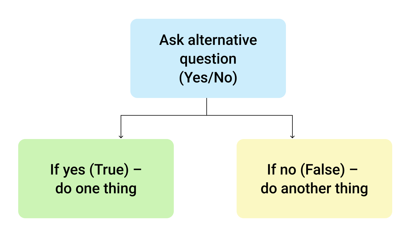
So, the IF function allows you to ask a question and indicate two alternative actions depending on the received answer. This question and the alternative actions are known as three arguments of the function.
IF function syntax in Google Sheets
The syntax for the IF function and its arguments are as follows:
- logical_expression – (required) a value or logical expression that is tested to see if it is TRUE or FALSE.
- value_if_true – (required) the operation that is carried out if the test is TRUE.
- value_if_false – (optional) the operation that is carried out if the test is FALSE.
Let's explore the arguments of our IF function in more detail.
The first argument represents a logical question. Google Sheets answers this question with either "yes" or "no", i.e. "true" or "false".
How to formulate the question properly, you may wonder? To do that, you can write a logical expression using such helpful symbols (or comparison operators) as "=", ">", "<", ">=", "<=", "<>". Let us try and ask such a question together.
Usage of the IF function
Let's assume that you are working in the company selling chocolate in several consumer regions with many clients.
This is what your sales data may look like in Google Sheets:
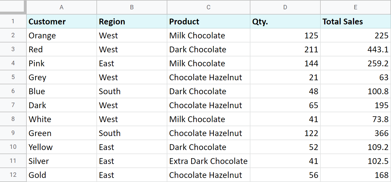
Imagine that you need to separate sales made in your local regions from those from abroad. To accomplish that, you should add another descriptive field for each sale – a country where the sales took place. Since there is a lot of data, you need this description field to be created automatically for each entry.
And this is when the IF function comes to play. Let's add the "Country" column to the data table. "West" region represents local sales (Our Country), while the rest are the sales from abroad (Rest of the World).
How to write out the function properly?
Place the cursor in F2 to make the cell active and type in the equality sign (=). Google Sheets will immediately understand that you are going to enter a formula. That's why right after you type the letter "i" it will prompt you to choose a function that begins with that same letter. And you should choose "IF".
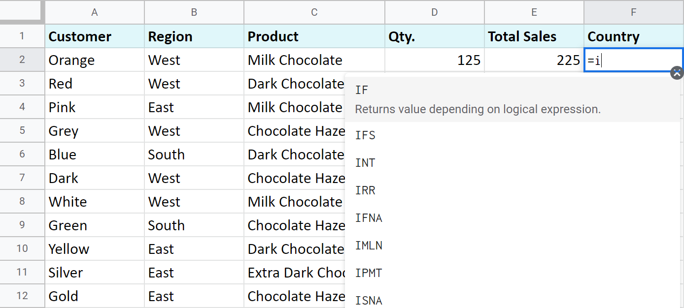
After that, all your actions will be accompanied by prompts as well.
For the first argument of the IF function, enter B2="West". As with the other Google Sheets functions, you don't need to enter the address of the cell manually – a mouse click is enough. Then enter comma (,) and specify the second argument.
The second argument is a value that F2 will return if the condition is met. In this case, it will be the text "Our Country".
And again, after the comma, write the value of the 3rd argument. F2 will return this value if the condition is not met: "Rest of the World". Do not forget to finish your formula entry by closing parenthesis ")" and pressing "Enter".
Your entire formula should look like this:
=IF(B2="West","Our Country","Rest of the World")
If everything is correct, F2 will return the text "Our Country":
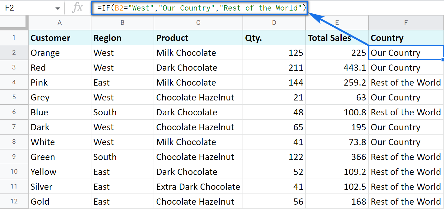
Now, all you have to do is to copy this function down column F.
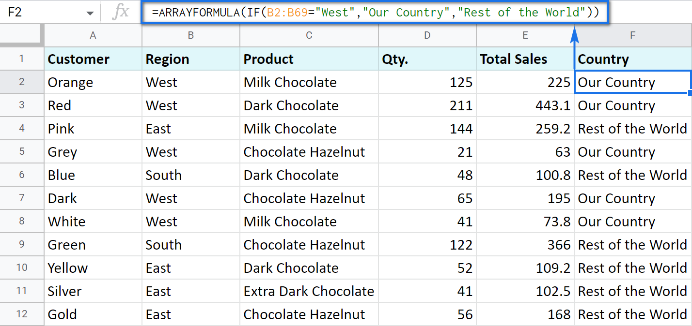
Tip. There's one way to process the entire column with one formula. The ARRAYFORMULA function will help you do that. Using it in the first cell of the column, you can test all cells below against the same condition, and return the corresponding result to each row at the same time:
=ARRAYFORMULA(IF(B2:B69="West","Our Country","Rest of the World"))
Let's examine the other ways of working with the IF function.
IF function and text values
The usage of the IF function with a text has already been illustrated in the example above.
Note. If the text is being used as the argument, then it must be enclosed in double-quotes.
IF function and numerical values
You can use numbers for the arguments just as you did with the text.
However, what is very important here is that the IF function makes it possible to not only fill cells with certain numbers based on the conditions met but also calculate.
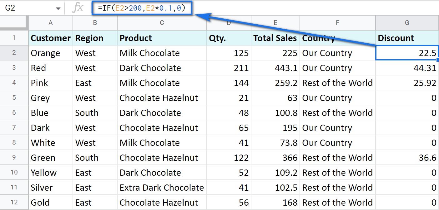
For example, let's say you offer your clients various discounts based on the total value of the purchase. If the total is more than 200, then the client gets a 10% discount.
For that, you need to use column G and name it "Discount". Then enter the IF function in G2, and the second argument will be represented by the formula that calculates the discount:
=IF(E2>200,E2*0.1,0)
IF blanks/non-blanks
There are cases when your result depends on whether the cell is empty or not. There are two ways to check that:
- Use the ISBLANK function.
For example, the following formula checks if cells in column E are empty. If so, no discount should be applied, otherwise, it's 5% off:
=IF(ISBLANK(E2)=TRUE,0,0.05)
Note. If there's a zero-length string in a cell (returned by some formula), the ISBLANK function will result in FALSE.
Here is another formula to check if E2 is empty:
=IF(ISBLANK(E2)2<>FALSE,0,0.05)You can turn the formula the other way around and see if cells are not blank instead:
=IF(ISBLANK(E2)=FALSE,0.05,0=IF(ISBLANK(E2)<>TRUE,0.05,0) - Use standard comparison operators with a pair of double-quotes:
Note. This method considers zero-length strings (indicated by double-quotes) as empty cells.
=IF(E2="",0,0.05)– check if E2 is blank=IF(E2<>"",0,0.05)– check if E2 is not empty.Tip. In a similar manner, use double-quotes as an argument to return an empty cell by the formula:
=IF(E2>200,E2*0,"")
IF in combination with other functions
As you have already learned, the text, numbers, and formulas can act as the arguments of the IF function. However, other functions can play that role as well. Let's see how it works.
Google Sheets IF OR
Remember the first way you figured out the country where you sold chocolate? You checked if B2 contained "West".
However, you can build the logic the other way around: list all the possible regions that belong to the "Rest of the World" and check if at least one of them appears in the cell. The OR function in the first argument will help you do that:
- logical_expression1 – (required) the first logical value to check for.
- logical_expression2 – (optional) the next logical value to check for.
- and so on.
As you can see, you just enter as many logical expressions as you need to check and the function searches if one of them is true.
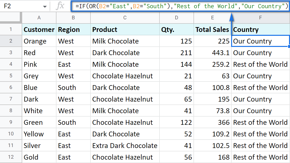
To apply this knowledge to the table with sales, mention all the regions that belong to the sales abroad, and the other sales will automatically become local:
=IF(OR(B2="East",B2="South"),"Rest of the World","Our Country")
Google Sheets IF AND
The AND function is just as simple. The only difference is that it checks if all listed logical expressions are true:
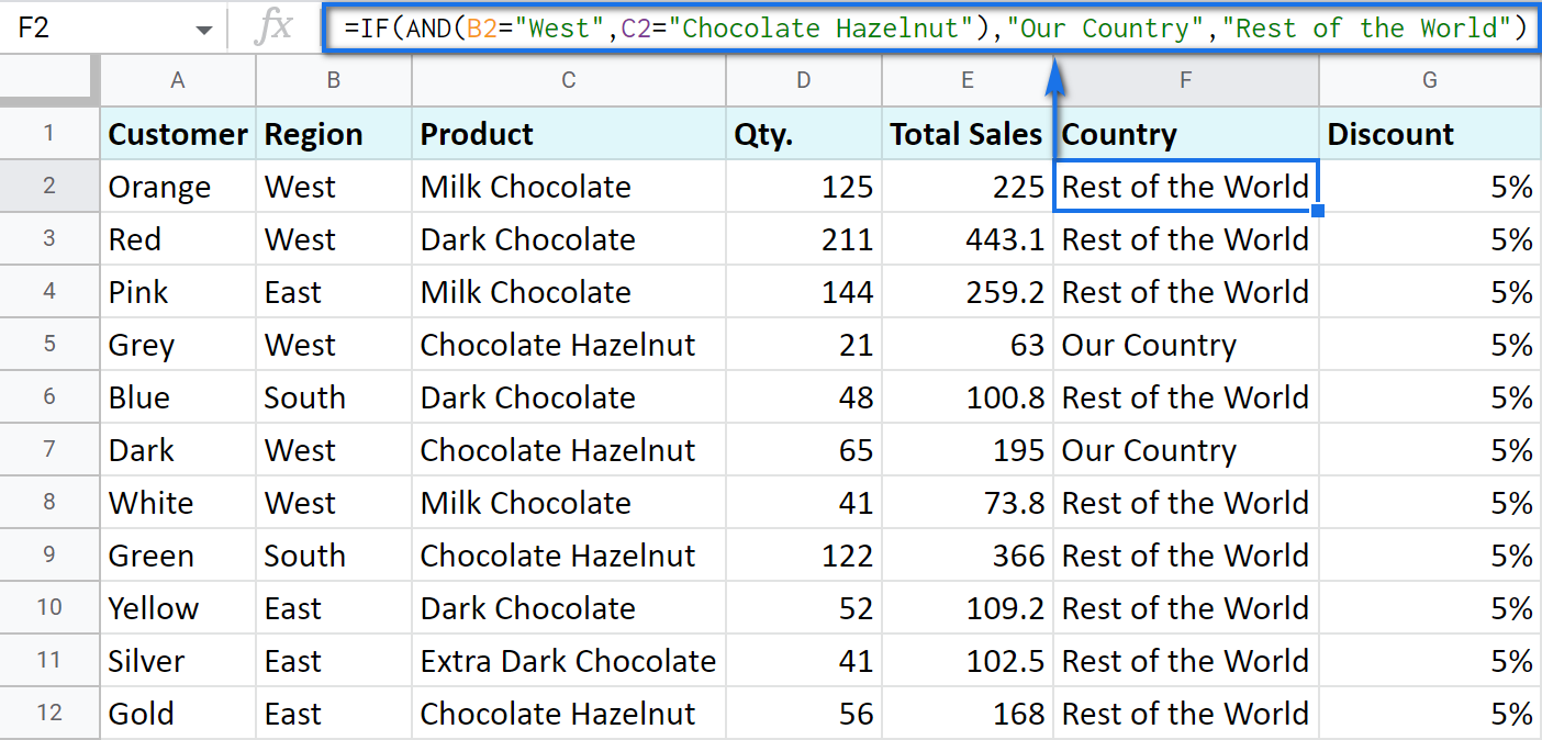
E.g. you need to narrow the search to your town and you know that it is currently buying only hazelnuts. So there are two conditions to consider: region – "West" and product – "Chocolate Hazelnut":
=IF(AND(B2="West",C2="Chocolate Hazelnut"),"Our Country","Rest of the World")
Nested IF formula vs. IFS function for Google Sheets
You can also use the IF function itself as an argument for the bigger IF function.
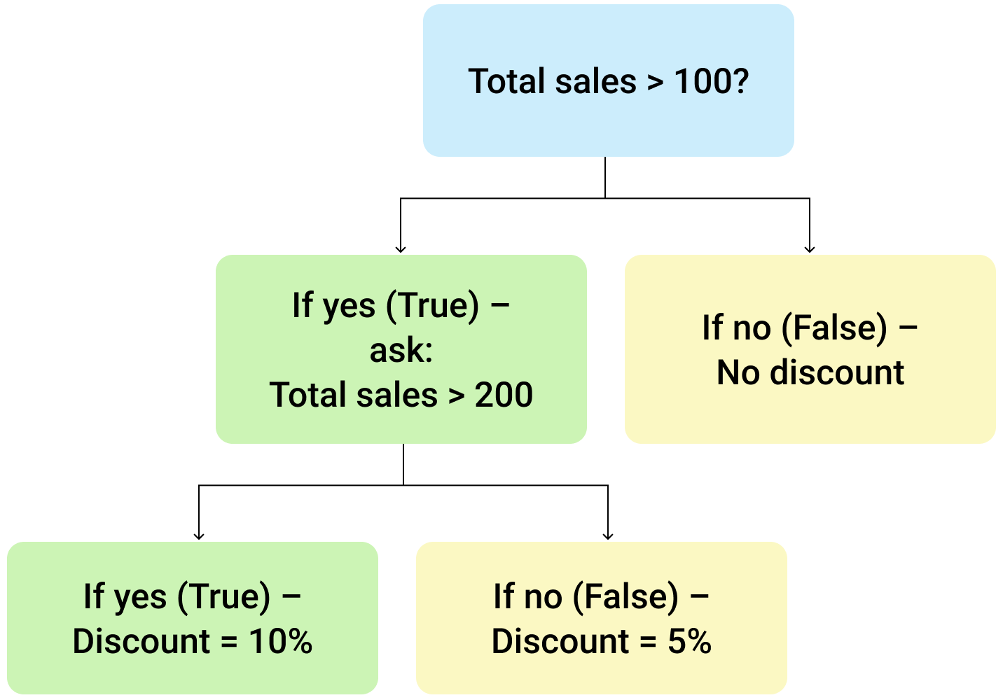
Let's assume that you have set stricter discount conditions for your clients. If the total purchase is more than 200 units, they get a 10% discount; if the total purchase is between 100 and 199, the discount is 5%. If the total purchase is lower than 100, there is no discount whatsoever.
The following formula shows how the function will look in the cell G2:
=IF(E2>200,E2*0.1,IF(E2>100,E2*0.05,0))
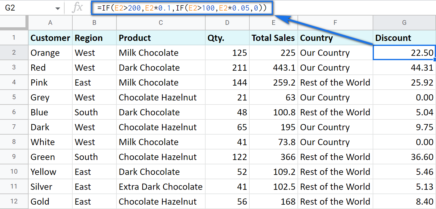
Note that it is another IF function that is used as the second argument. In such cases, the decision tree is as follows:
Let's make it even more fun and complicate the task. Imagine that you're offering the discounted price to the one region only - "East".
To do that correctly, add the logical expression "AND" to our function. The formula will then look the following way:
=IF(AND(B2="East",E2>200),E2*0.1,IF(AND(B2="East",E2>100),E2*0.05,0))
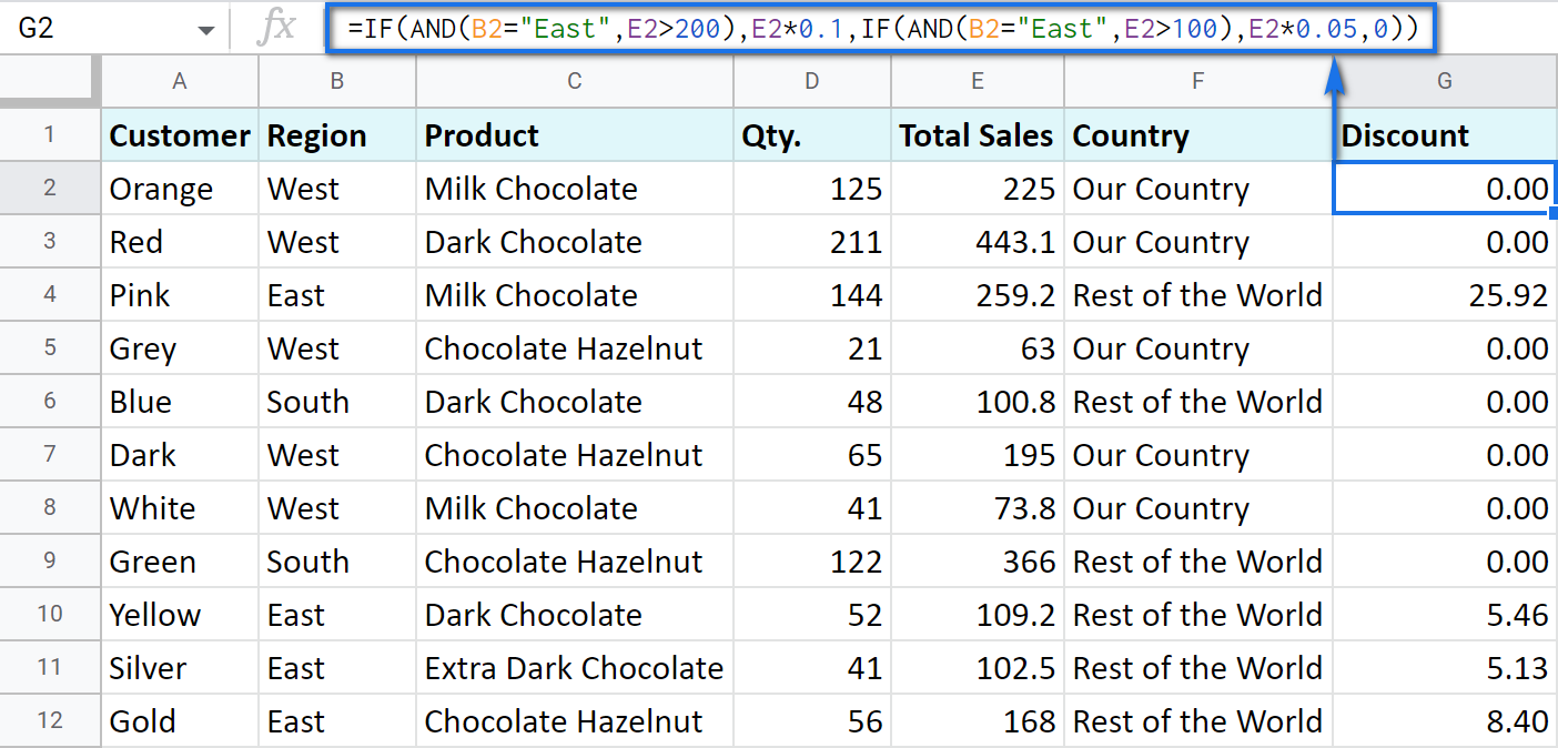
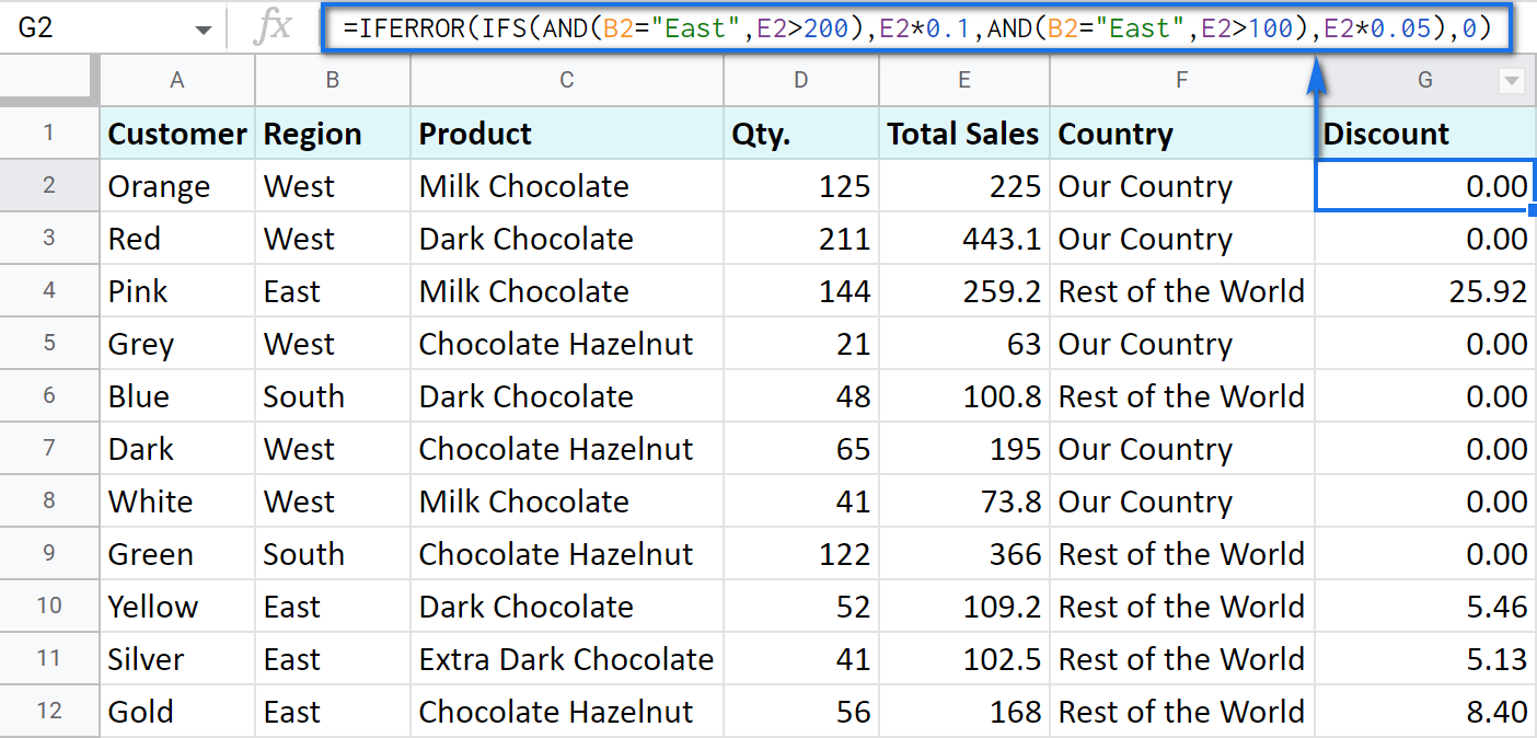
As you can see, the number of discounts has reduced greatly while their amount remains intact.
There's also an easier way to write the above thanks to the IFS function:
- condition1 – (required) is the logical expression you want to test.
- value1 – (required) is the value to return if the condition1 is true.
- and then you just list conditions with their values to return if they are true.
Here's how the above formula will look with IFS:
=IFS(AND(B2="East",E2>200),E2*0.1,AND(B2="East",E2>100),E2*0.05)
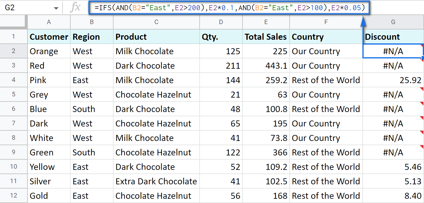
Tip. If there's no true condition, the formula will return the #N/A error. To avoid that, wrap your formula with IFERROR:
=IFERROR(IFS(AND(B2="East",E2>200),E2*0.1,AND(B2="East",E2>100),E2*0.05),0)
SWITCH as an alternative to multiple IFs
There's one more function you may want to consider instead of the nested IF: Google Sheets SWITCH.
It checks if your expression corresponds to a list of cases, one by one. When it does, the function returns a corresponding value.
- expression is any cell reference, or a range of cells, or even an actual math expression, or even a text that you'd like to equal to your cases (or test against the criteria). Required.
- case1 is your first criteria to check the expression against. Required.
- value1 is a record to return if the case1 criterion is the same as your expression. Required.
- case2, value2 repeat as many times as criteria you have to check and values to return. Optional.
- default is also completely optional. Use it to see a specific record if none of the cases is met. I'd recommend using it every time to avoid errors when your expression doesn't meet matches among all the cases.
Here are a couple of examples.
To test your cells against a text, use ranges as an expression:
=ARRAYFORMULA(SWITCH(B2:B69,"West","Our Country","Rest of the World"))
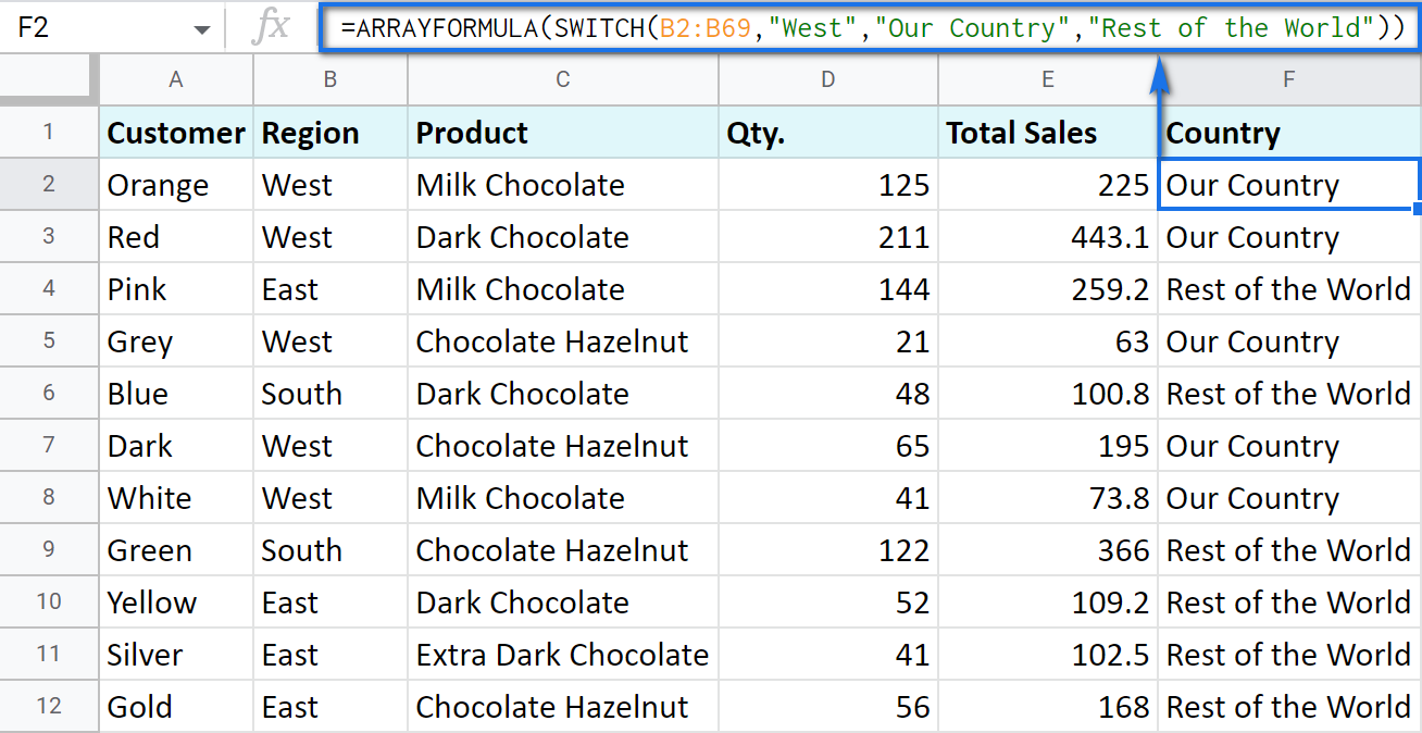
In this formula, SWITCH checks what record is in every cell in column B. If it's West, the formula says Our Country, otherwise, Rest of the World. ArrayFormula makes it possible to process the entire column at once.
To work with calculations, it's better to use a boolean expression:
=SWITCH(TRUE,$E2>200,$E2*0.1,AND($E2<200,$E2>100),$E2*0.05,0)
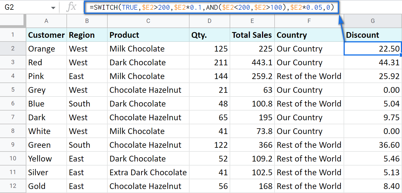
Here SWITCH checks if the result of the equation is TRUE or FALSE. When it's TRUE (like if E2 is really greater than 200), I get a corresponding result. If none of the cases in the list is TRUE (meaning they are FALSE), the formula simply returns 0.
Note. SWITCH doesn't know how to calculate the entire range at once, so no ARRAYFORMULA in this case.
IF statements based on a count
One of the questions we get asked a lot is how to create the IF formula that will return whatever you need if the column contains or doesn't contain a certain record.
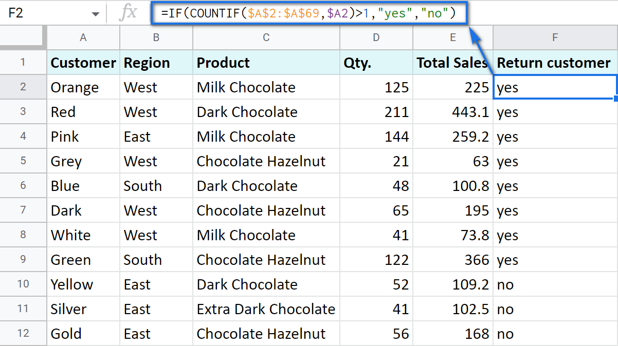
For example, check if a customer's name appears more than once in a list (column A) and put the corresponding word (yes/no) into a cell.
A solution is simpler than you may think. You need to introduce the COUNTIF function to your IF:
=IF(COUNTIF($A$2:$A$69,$A2)>1,"yes","no")
Make Google Sheets build IF formulas for you – IF Formula Builder add-on
If you're tired of keeping track of all those extra characters and proper syntax in formulas, there's another solution available.
IF Formula Builder add-on for Google Sheets offers a visual way of creating IF statements. The tool will handle syntax, extra functions and all required characters for you.
All you need to do is:
- fill blanks with your records one by one. No special treatment for dates, time, etc. Enter them as you always do and the add-on will recognize the data type.
- select required comparison operators from the suggested drop-down lists.
- if needed, add multiple logical expressions in a click: IF OR, IF AND, ELSE IF, THEN IF.
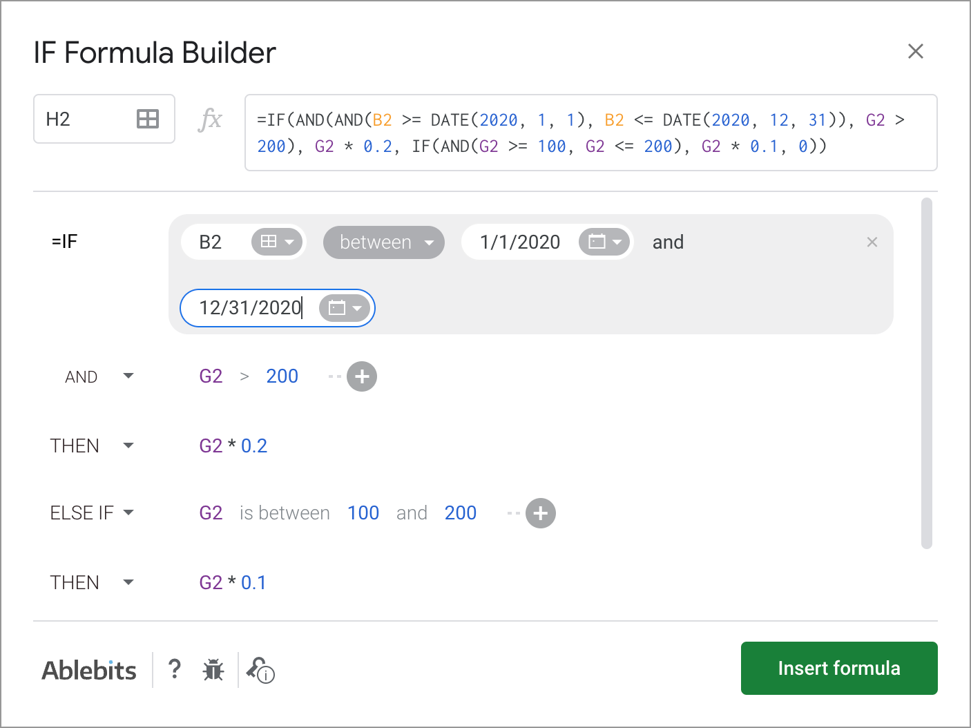
As you can see, each logical expression takes its own line. The same goes for true/false outcomes. This reduces the number of possible confusion over the formula drastically.
As you fill everything out, the formula for use will grow in the preview area at the top of the window. To its left, you can select a cell in your sheet where you'd like to have the formula.
When you're ready, paste the formula into the cell of interest by clicking the Insert formula button at the bottom.
Please visit the online tutorial for IF Formula Builder to see all options described in detail.
I hope that there's no room for any doubt now that the IF function, though a very simple one at first glance, opens the door to many options for data processing in Google Sheets. But if you still have questions, feel free to ask them in the comments section down below – we'll be happy to help!
 by
by
607 comments
Im trying to do an if statment that will allow the cell to change fill color on sheets. I have figured out the if, now i just need something like a than. Any thoughts on what i should do?
Hello Nickyc,
The IF function is usually used to return values into cells. If your task is to color cells differently based on various conditions, you need to create a couple of conditional formatting rules. Please refer to this article to check how to do that correctly.
How do I get the value of F2, to show up in H2, when G2 is blank? It is showing up FALSE currently.
=IF(OR(G2=5,G2=10,G2=15),"NT", IF(G2="BLANK",F2))
Nikki,
here's a formula for you to try in H2:
=IF(OR(G2=5,G2=10,G2=15),"NT",IF(ISBLANK(G2)=TRUE,F2,""))
Data from a sheet which has data of two products. The graphs for both products need to be different. How is this possible? the graph plotted for the value of a certain value in the graph. the sheet contacts a column for product and for the value specified in the previous sentence.
Hi Kowshik,
I'm sorry but your task is not clear. If you're having difficulties with charts in Google Sheets, I'd recommend you to check out the corresponding article - about charts in Google Sheets.
Hi I need a formula for if column A is populated (by a date), then column D will show a date 3 days later and column E will show a date 21 days later. Can this be done?
Hi Janel,
If I understand your task correctly and cells in column A contain either date or nothing at all, the following formula will do for column D (assuming the data starts from the second row):
=IF(ISBLANK($A2),"",$A2+3)
And here's the one for column E:
=IF(ISBLANK($A2),"",$A2+21)
You need to copy the formula down to other rows. The formulas won't return anything if cells in A are blank.
Or you can use the array formula like this in D2 (adjust accordingly for E2):
=ARRAYFORMULA(IF(ISBLANK($A:$A),"",$A:$A+3))
It will automatically calculate the result for each row of your table.
Couldn't find an example like the situation I'm in, so what I'm looking to do is see how many instances of a cell exist in a range based on if an associate of that cell equals a specific phrase, in essence I'm looking to do something like this; if(A2,"Phrase") then countif($A$3:$A$1500,A3). I keep running into a different size error, any thoughts on how what I'm looking to do could be done?
I tried to build a sample formula based on what you described, and this one worked for me:
=IF(A2="Phrase",COUNTIF($A$3:$A$1000,A3),"")
Please specify if I've got something wrong.
I have a spreadsheet of data based on testing of kids. I have the cells programmed to meet our criteria =IF(AND(F5>80%, G5>=1, H5>=1), "X" , " ") My problem is that the next three columns =IF(AND(F5>80%, G5>=1, H5>=1), "X" , " ") build on that same data and I can't figure out how to only have one column with an "X" Ideally, I would only like the highest column to have the X, not all. Thank you for any help you can share.
Correction: The first column has: =IF(AND(F5>80%, G5>=1, H5>=1), "X" , " ")
The second column has: =IF(AND(F5=100%, G5>=2, H5>=2), "X" , " ")
As you can see, if I child had 100% in F5, they meet the criteria for both columns, but we really only want the highest one to have the "X".
I believe adjusting the condition a bit will help you. You need to exclude that 100% from your first formula. Just add one more AND that will check that F5 is both greater than 80 but less than 100:
=IF(AND(AND(F5>80%,F5<100%),G5>=1,H5>=1),"X","")
Hope this helps.
How do I apply this formula to every cell in a column?
I.E. If any cell in column A says "this" then the cell adjacent, in Column B would say "that"
Either enter the formula to the first cell and then copy it down all other rows, or use the array formula like this:
=ARRAYFORMULA(IF($A:$A="this","that",""))
I'm quite new to Google Sheets, but understand If/Then from another software. May I ask if there is a way to use IF to populate a new sheet? Meaning, if the cell has x, then the contents of that row should copy to another spreadsheet?
There's a special IMPORTRANGE function that helps to return the entire range of cells from another sheet. Here's an example formula for you:
=IF(Sheet2!A2="X",IMPORTRANGE("spreadsheet_url","Sheet1!A2:Z2"),"")
Hope this will help.
If I have a numerical value of 38 in A1. And I want a factor of 8.2 to show up in B1 it would be written as follows;
=IF(A10=38,8.2)
But what if I had multiple rows with different numerical values and I wanted a factor based on the numerical value as follows;
A B C D
1 40 8.8
2 42 9.0
3 44 9.5
4 46 10.0
If I enter 44 in column A it would enter a factor of 9.5 in column B. If I enter 42 in column A it would enter a factor of 9.0 in column B. How would I formulate that?
The last point of the article above mentions this. Look for "argument for the bigger IF function".
Hi,
Great article! Many thanks. Although good examples, unfortunately I wasn't able to successfully apply them to my sheet.
I'm trying to apply the following logic:
If H24 = smaller than 68600, then H24*36,93%, If H24 = > 68600 then take maximum 68600 * 36,93%
And in the next cell:
If H24 = > 68600, then (H24-68600)*50,5%
Can you help with the formulas for this?
Many thanks in advance
Hi Jeffrey,
I believe you need to simply switch "=" and ">". Also, make sure you separate percentage decimals by a full stop rather than a comma. The correct formula would be:
=IF(H24<68600,H24*36.93%,IF(H24>=68600,68600*36.93%,""))
I guess the same mistakes were made in the second formula. Will you be able to adjust it based on my example? ;)
Hi,
Is it possible to give an IF to more than 1 rule at the same time?
I'm trying to create a formula to calculate someone's commission in Google.Doc's
The rule is if they reach their 100% target, the Sales £ they have earned will be multiplied by 1%. IF they exceed their target (E.G they achieved 125% of their target). the 100% achieved will still be multiplied by 1% but the extra 25% they earned will be multiplied by 1.25%. How do you make it so ONLY 100%> is at the higher rate of 1.25%
I've gotten this far so far: =IF(B7>1,(B6*1%)
Thank you
Hi, Jamie. You need a nested if. Look:
=IF(AND(B7>1, B71.25, B6*1.25%))
been trying to make a formula in google sheets
what I want to make is there should be a dropdown menu for Yes or No, but only if another cell in another sheet says No, because if that one says Yes there shouldn't be a dropdown menu and it should just say Yes. And the opposite is also true. Of course it would be cool if the dropdown menu still works and it's just linked to that other cell.
What does work is
=IF('Side Quests'!A50="Yes";"Yes";"No")
but then I can't use the dropdown menu anymore and that would mean I can only change the value on that one sheet and not on the one where this formula is. Is there something that I'm missing here? Is it possible to link both cells to eachother, in a way that they both have the same dropdown menu, and if you change one, the other will change to the same?
Thanks in advance ^^
I'm afraid you won't be able to do that with basic formulas. You need to use scripts to solve the task.
You may try to find the solution here - an overview of Google Apps Script with a lot of helpful content and links.
I have a google form that submits the email address of the user and enters it to field A2. I have another field, B2 that is calculated to capture that email address. The problem: The form goes through 3 levels for approval, and at each level the email is captured and replaces the information in field A2. My goal is to capture the applicant email address, which is the first email entered.
I am also using an arrayfunction that completes all rows. I can't figure out how to make it only get the first entry. Can you help?
Clarification: My goal is to capture the applicant email address, which is the first email entered in A2 by copying it to B2 and not have B2 change again when A2 captures the next email address in A2.
Hello, Brenda,
I'm sorry, but there's no way to prevent formulas in Google Sheets from recalculating. There are a couple of spreadsheet settings that can reduce the number of recalculations, but only for few formulas. You can check the list by going to File > Spreadsheet settings > Calculations.
I wish I could help you better.
thanks
I am trying to make a formula for my math teacher to do grades on Google Sheets. I am trying to accomplish the following: If column B has the text "A-" or "A" or A+", then column C should be filled with the number 4, if column B has the text "B-" or "B" or B+", then column C should be filled with the number 3, if column B has the text "C-" or "C" or C+", then column C should be filled with the number 2, if column B has the text "D-" or "D" or D+", then column C should be filled with the number 1, and if column B has the text "F-" or "F" or F+", then column C should be filled with the number 0.
Thank you for the detailed description of the task, Tarun.
If you'd like to do that with the IF function, put the following to C2 and copy the formula down (assuming the data in column B starts in B2):
=IF(LEFT(B2,1)="A",4,IF(LEFT(B2,1)="B",3,IF(LEFT(B2,1)="C",2,IF(LEFT(B2,1)="D",1,IF(LEFT(B2,1)="F",0,"")))))
Alternatively, you could create a "helper table", where column E would contain the list of all grades, and column F would have corresponding grades. Then, the following should also do:
=VLOOKUP(B1,$E$1:$F$15,2,FALSE)
Hope these formulas help!
Can you help me write a correct formula?
Calculate percentage of difference between two cells when both cells are non-zero.
Currently have the following but getting error - not sure how to check for non-zero cells and only proceed with calculation when they are.
=IF ((G419>0)AND(G445>0)),(((G445-G419)/G445)*100)
Thank you!
Cathy,
Please try the following:
=IF(AND(G419>0,G445>0),((G445-G419)/G445)*100,"")
If you'd like to know how to build the formula like this correctly, please look through this article. It's written for Excel, but the function works the same in Google Sheets.
Hope this helps!
I have a column in my sheet containing fares that I want to auto-populate based on a vehicle type AND a route:
Column A : vehicle
Column B: route
Column C: fare
Routes originating at an airport (but not a specified airport) cost more than others so the formula I am trying to use (in column C) but gives #ERROR! is:
=if(AND((A1="Sedan",B2="%Airport%"),"$350","$330", if(AND((A1="SUV",B2="%Airport%"),"$400","$350", if(AND((A1="minibus",B2="%Airport%"),"$$550","$500"))))))
If anyone can help me out with where the parse error is that would be awesome.
Thanks!
Thank you for contacting us, Kate.
First, if you want to check for any airport occurrences, you need to use the ISNUMBER+SEARCH combo instead of wildcard characters.
Also, you used one excess opening bracket for your AND functions. It should be like this:
AND(A2="Sedan",ISNUMBER(SEARCH("airport",B2)))
Once you fix that, the formula will return another error because you used more arguments than the function allows. You see, if your first condition is met, the formula will return $350, if not - $330. That's it, this is the formula.
In order to check other conditions, you need to replace all the second numbers with your next IFs:
=IF(AND(A2="Sedan",ISNUMBER(SEARCH("airport",B2))),"$350",IF(AND(A2="SUV",ISNUMBER(SEARCH("airport",B2))),"$400",IF(AND(A2="minibus",ISNUMBER(SEARCH("airport",B2))),"$$550","$500")))
If this is not what you need, please send me the example of your table (10-20 rows) to support@ablebits.com with the link to this comment.
I'll do my best to advise you.
Hello, Sean:
Try this:
=IF(ISBLANK(Inventory wk5!I2),Inventory wk5!I2,Inventory wk4!I2)
The ISBLANK function tests to see if the cell is empty, which is what I think you're testing. If you want to see if the cell is 0 then the formula should say =0. The zero character is a character and the cell would not be empty. Same thing for non-printing characters in cells. Those cells are not empty.
I am trying to create a formula to reference a cell from one sheet (if filled) or another sheet (if the first is not filled). This is what I have and it is not working.
=IF('Inventory wk 5'!I2>=0,'Inventory wk 5'!I2,'Inventory wk 4'!I2)
Anne:
Where column 1 is column A and the data is in A2 enter this in column 2:
=IF(A2<=40,A2,40)
I have a super simple scenario but don't know how to do this. I have 2 columns and I want column 2 to be: 'If the value in column 1 is less than 40, the column 1 value should appear as is. If the value is above 40, then the number 40 should appear. Any help would be appreciated! Thank you!