The IF function in Google Sheets is one of the easiest functions to learn, and while this holds true, it is also a very helpful one.
In this tutorial, I invite you to take a closer look at how Google Spreadsheet IF function works and what advantages you will get from using it.
What is the IF function in Google Sheets?
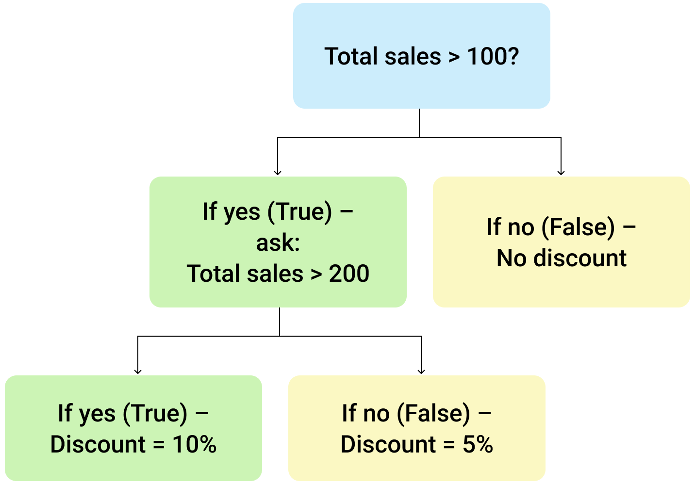
Whenever you use the IF function, you create a decision tree in which certain action follows under one condition, and if that condition is not met – another action follows.
For this purpose, the condition of the function must be in a format of the alternative question with only two possible answers: "yes" and "no".
This is what a decision tree may look like:
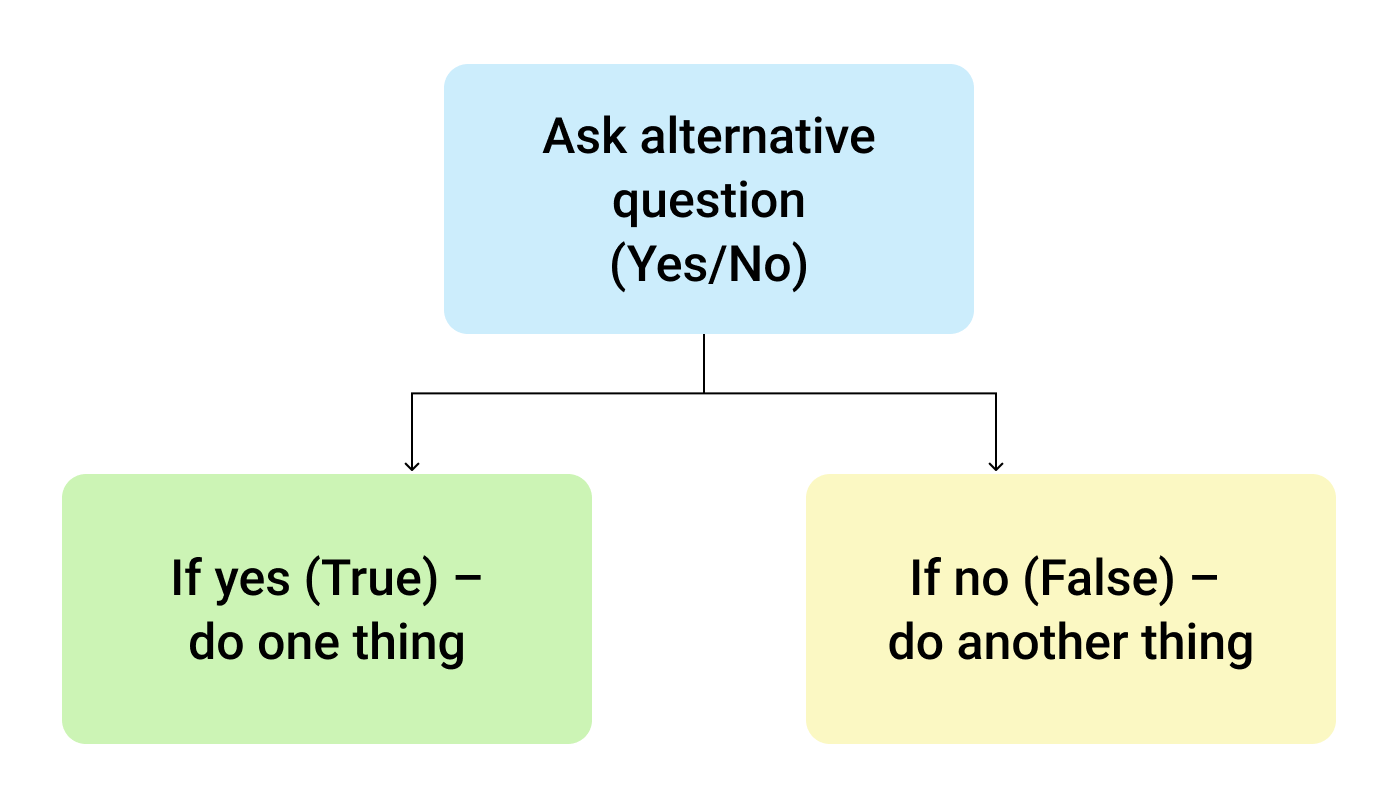
So, the IF function allows you to ask a question and indicate two alternative actions depending on the received answer. This question and the alternative actions are known as three arguments of the function.
IF function syntax in Google Sheets
The syntax for the IF function and its arguments are as follows:
- logical_expression – (required) a value or logical expression that is tested to see if it is TRUE or FALSE.
- value_if_true – (required) the operation that is carried out if the test is TRUE.
- value_if_false – (optional) the operation that is carried out if the test is FALSE.
Let's explore the arguments of our IF function in more detail.
The first argument represents a logical question. Google Sheets answers this question with either "yes" or "no", i.e. "true" or "false".
How to formulate the question properly, you may wonder? To do that, you can write a logical expression using such helpful symbols (or comparison operators) as "=", ">", "<", ">=", "<=", "<>". Let us try and ask such a question together.
Usage of the IF function
Let's assume that you are working in the company selling chocolate in several consumer regions with many clients.
This is what your sales data may look like in Google Sheets:
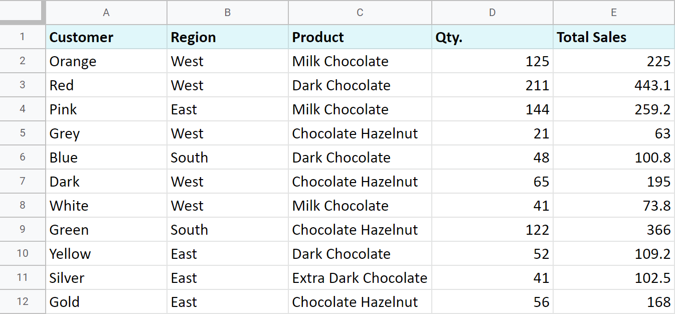
Imagine that you need to separate sales made in your local regions from those from abroad. To accomplish that, you should add another descriptive field for each sale – a country where the sales took place. Since there is a lot of data, you need this description field to be created automatically for each entry.
And this is when the IF function comes to play. Let's add the "Country" column to the data table. "West" region represents local sales (Our Country), while the rest are the sales from abroad (Rest of the World).
How to write out the function properly?
Place the cursor in F2 to make the cell active and type in the equality sign (=). Google Sheets will immediately understand that you are going to enter a formula. That's why right after you type the letter "i" it will prompt you to choose a function that begins with that same letter. And you should choose "IF".
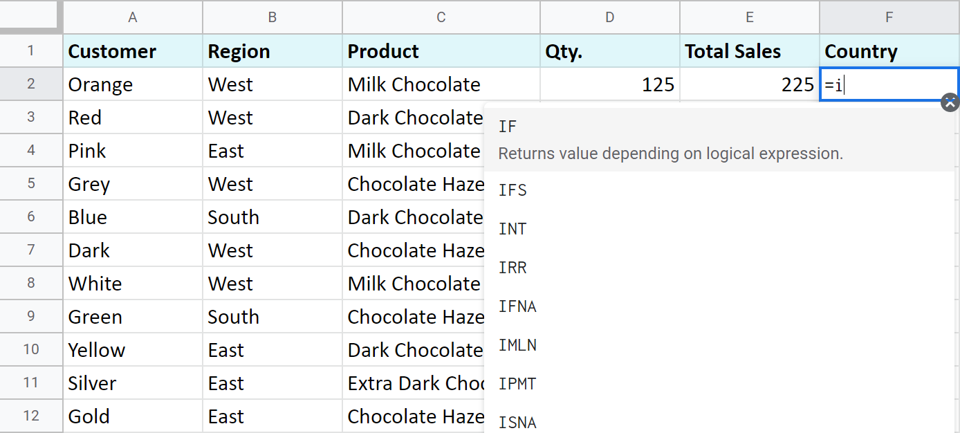
After that, all your actions will be accompanied by prompts as well.
For the first argument of the IF function, enter B2="West". As with the other Google Sheets functions, you don't need to enter the address of the cell manually – a mouse click is enough. Then enter comma (,) and specify the second argument.
The second argument is a value that F2 will return if the condition is met. In this case, it will be the text "Our Country".
And again, after the comma, write the value of the 3rd argument. F2 will return this value if the condition is not met: "Rest of the World". Do not forget to finish your formula entry by closing parenthesis ")" and pressing "Enter".
Your entire formula should look like this:
=IF(B2="West","Our Country","Rest of the World")
If everything is correct, F2 will return the text "Our Country":
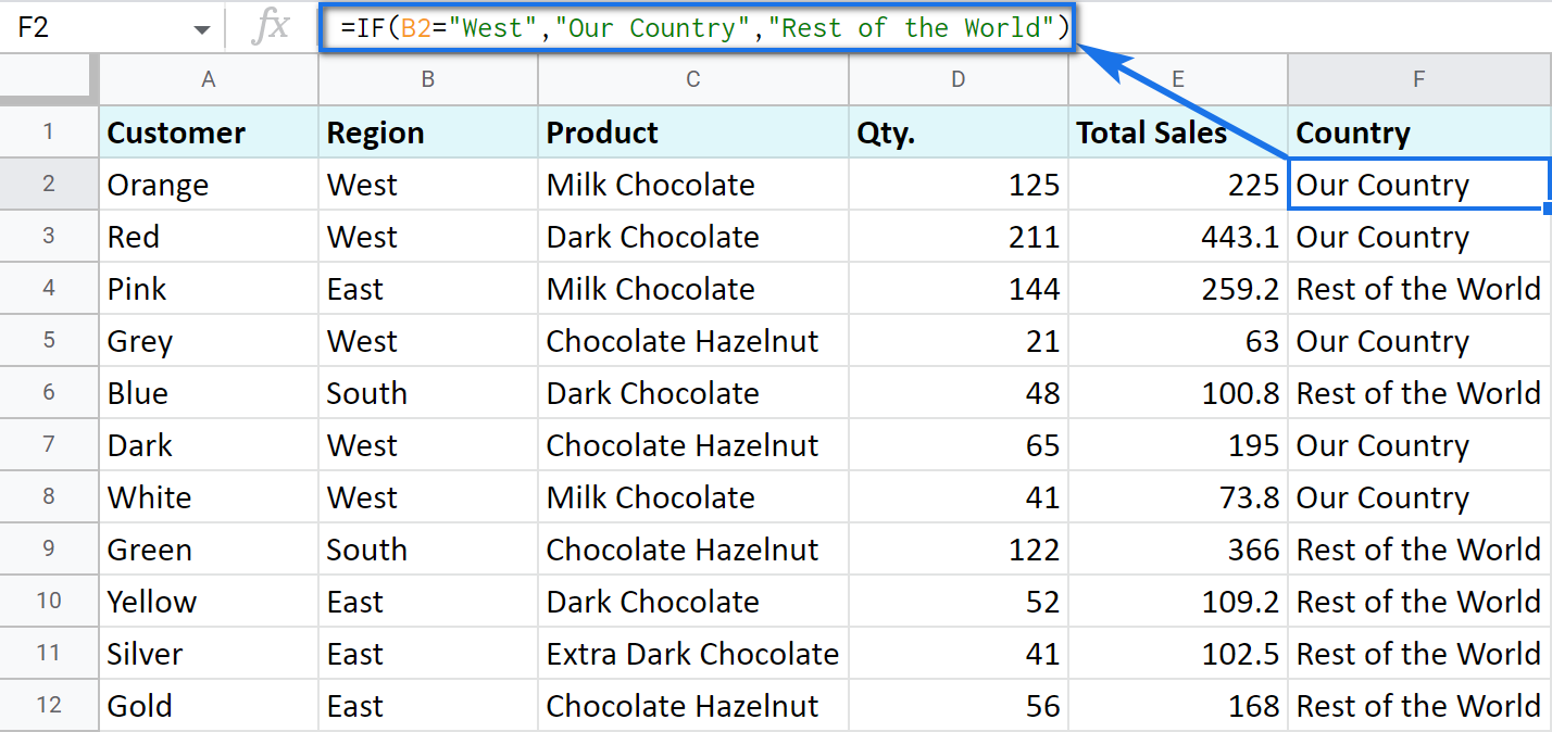
Now, all you have to do is to copy this function down column F.
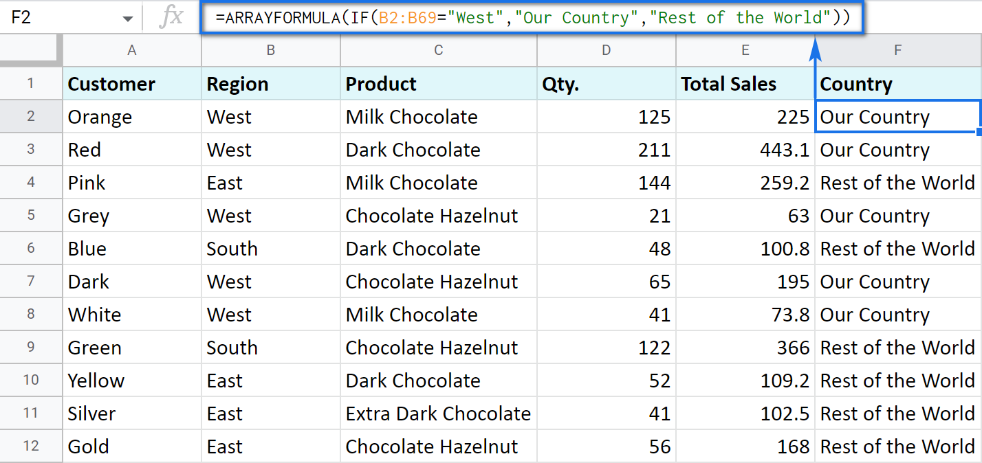
Tip. There's one way to process the entire column with one formula. The ARRAYFORMULA function will help you do that. Using it in the first cell of the column, you can test all cells below against the same condition, and return the corresponding result to each row at the same time:
=ARRAYFORMULA(IF(B2:B69="West","Our Country","Rest of the World"))
Let's examine the other ways of working with the IF function.
IF function and text values
The usage of the IF function with a text has already been illustrated in the example above.
Note. If the text is being used as the argument, then it must be enclosed in double-quotes.
IF function and numerical values
You can use numbers for the arguments just as you did with the text.
However, what is very important here is that the IF function makes it possible to not only fill cells with certain numbers based on the conditions met but also calculate.
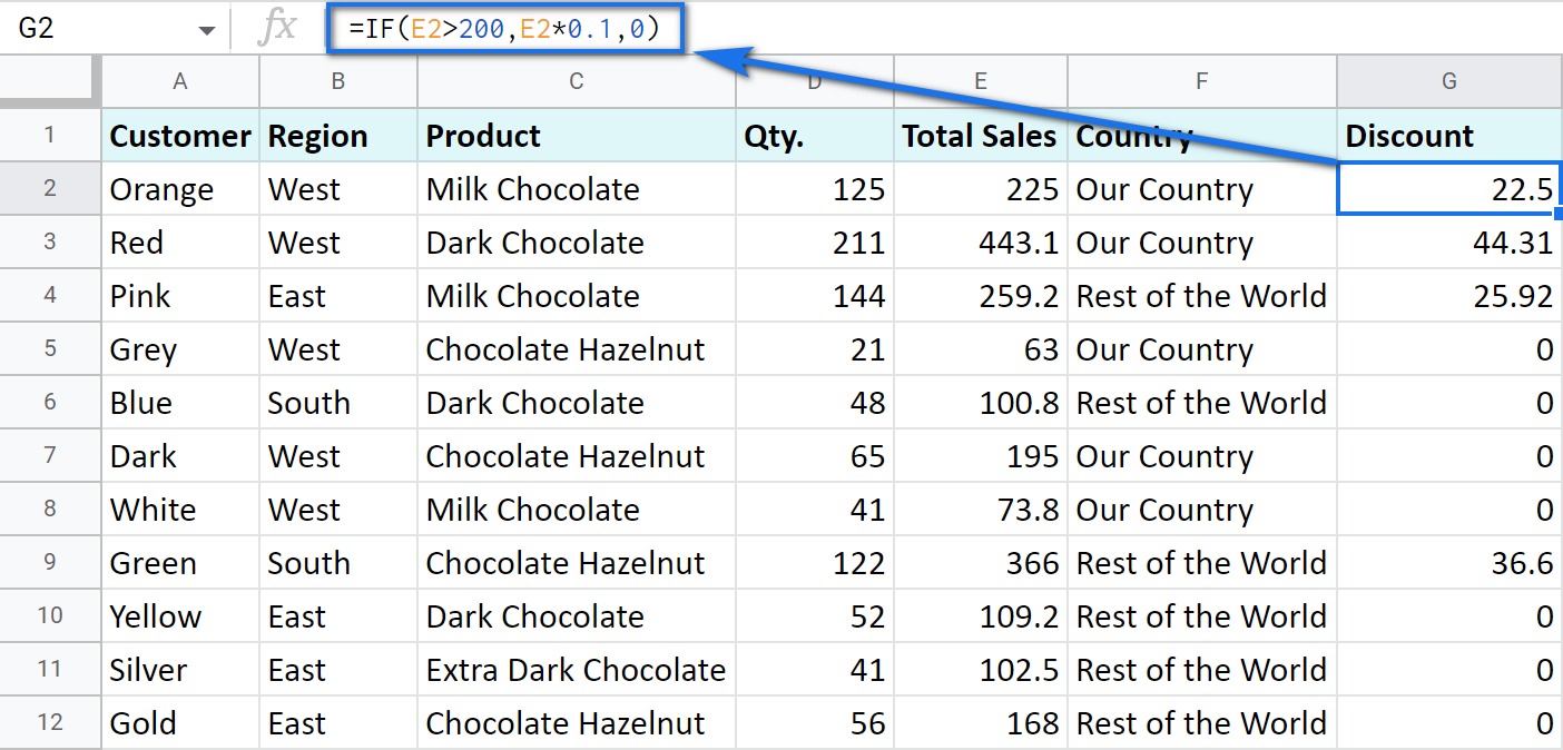
For example, let's say you offer your clients various discounts based on the total value of the purchase. If the total is more than 200, then the client gets a 10% discount.
For that, you need to use column G and name it "Discount". Then enter the IF function in G2, and the second argument will be represented by the formula that calculates the discount:
=IF(E2>200,E2*0.1,0)
IF blanks/non-blanks
There are cases when your result depends on whether the cell is empty or not. There are two ways to check that:
- Use the ISBLANK function.
For example, the following formula checks if cells in column E are empty. If so, no discount should be applied, otherwise, it's 5% off:
=IF(ISBLANK(E2)=TRUE,0,0.05)
Note. If there's a zero-length string in a cell (returned by some formula), the ISBLANK function will result in FALSE.
Here is another formula to check if E2 is empty:
=IF(ISBLANK(E2)2<>FALSE,0,0.05)You can turn the formula the other way around and see if cells are not blank instead:
=IF(ISBLANK(E2)=FALSE,0.05,0=IF(ISBLANK(E2)<>TRUE,0.05,0) - Use standard comparison operators with a pair of double-quotes:
Note. This method considers zero-length strings (indicated by double-quotes) as empty cells.
=IF(E2="",0,0.05)– check if E2 is blank=IF(E2<>"",0,0.05)– check if E2 is not empty.Tip. In a similar manner, use double-quotes as an argument to return an empty cell by the formula:
=IF(E2>200,E2*0,"")
IF in combination with other functions
As you have already learned, the text, numbers, and formulas can act as the arguments of the IF function. However, other functions can play that role as well. Let's see how it works.
Google Sheets IF OR
Remember the first way you figured out the country where you sold chocolate? You checked if B2 contained "West".
However, you can build the logic the other way around: list all the possible regions that belong to the "Rest of the World" and check if at least one of them appears in the cell. The OR function in the first argument will help you do that:
- logical_expression1 – (required) the first logical value to check for.
- logical_expression2 – (optional) the next logical value to check for.
- and so on.
As you can see, you just enter as many logical expressions as you need to check and the function searches if one of them is true.
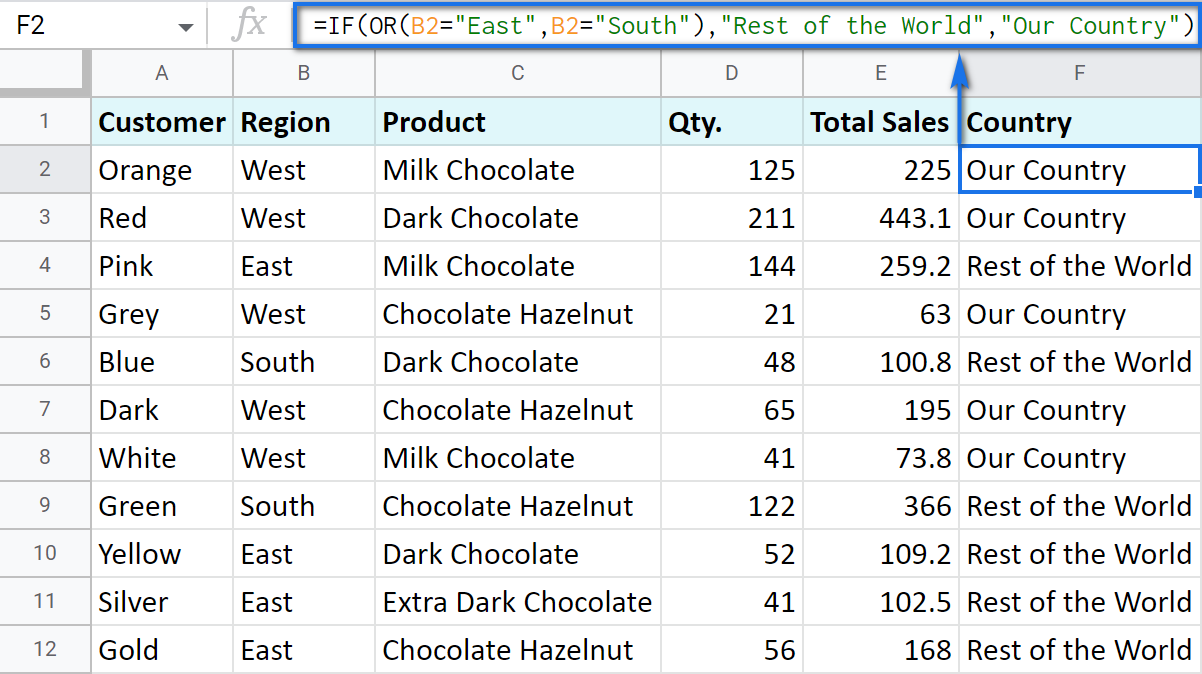
To apply this knowledge to the table with sales, mention all the regions that belong to the sales abroad, and the other sales will automatically become local:
=IF(OR(B2="East",B2="South"),"Rest of the World","Our Country")
Google Sheets IF AND
The AND function is just as simple. The only difference is that it checks if all listed logical expressions are true:
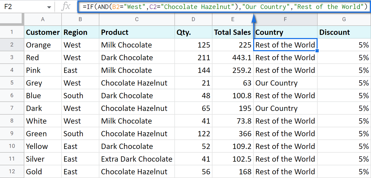
E.g. you need to narrow the search to your town and you know that it is currently buying only hazelnuts. So there are two conditions to consider: region – "West" and product – "Chocolate Hazelnut":
=IF(AND(B2="West",C2="Chocolate Hazelnut"),"Our Country","Rest of the World")
Nested IF formula vs. IFS function for Google Sheets
You can also use the IF function itself as an argument for the bigger IF function.
Let's assume that you have set stricter discount conditions for your clients. If the total purchase is more than 200 units, they get a 10% discount; if the total purchase is between 100 and 199, the discount is 5%. If the total purchase is lower than 100, there is no discount whatsoever.
The following formula shows how the function will look in the cell G2:
=IF(E2>200,E2*0.1,IF(E2>100,E2*0.05,0))
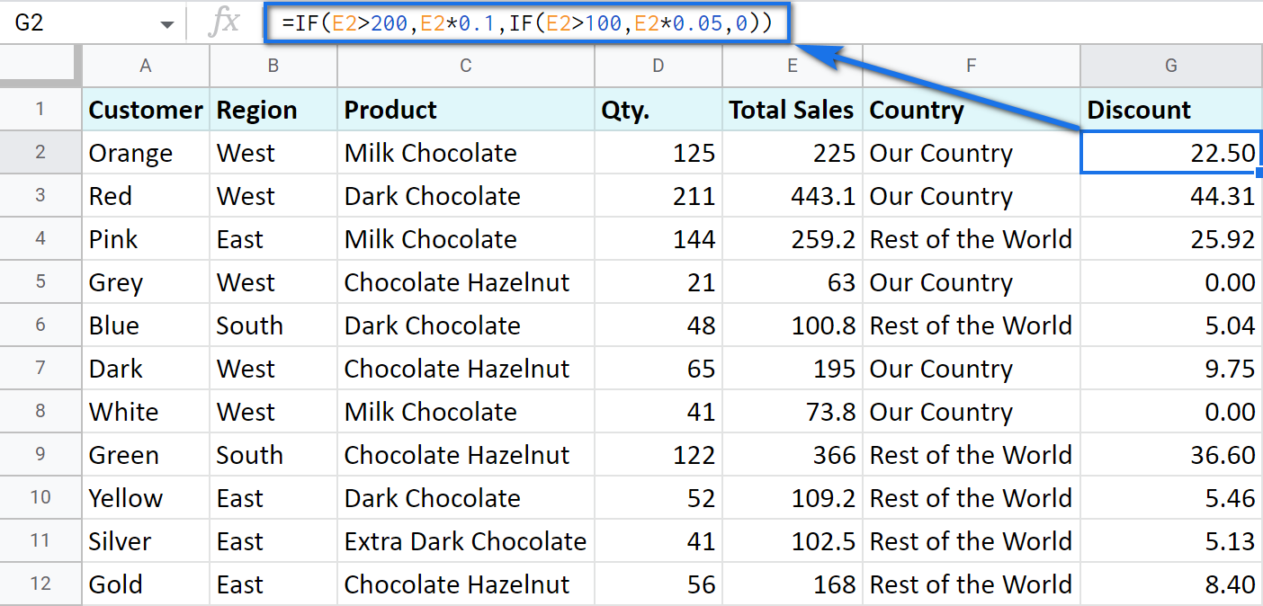
Note that it is another IF function that is used as the second argument. In such cases, the decision tree is as follows:
Let's make it even more fun and complicate the task. Imagine that you're offering the discounted price to the one region only - "East".
To do that correctly, add the logical expression "AND" to our function. The formula will then look the following way:
=IF(AND(B2="East",E2>200),E2*0.1,IF(AND(B2="East",E2>100),E2*0.05,0))
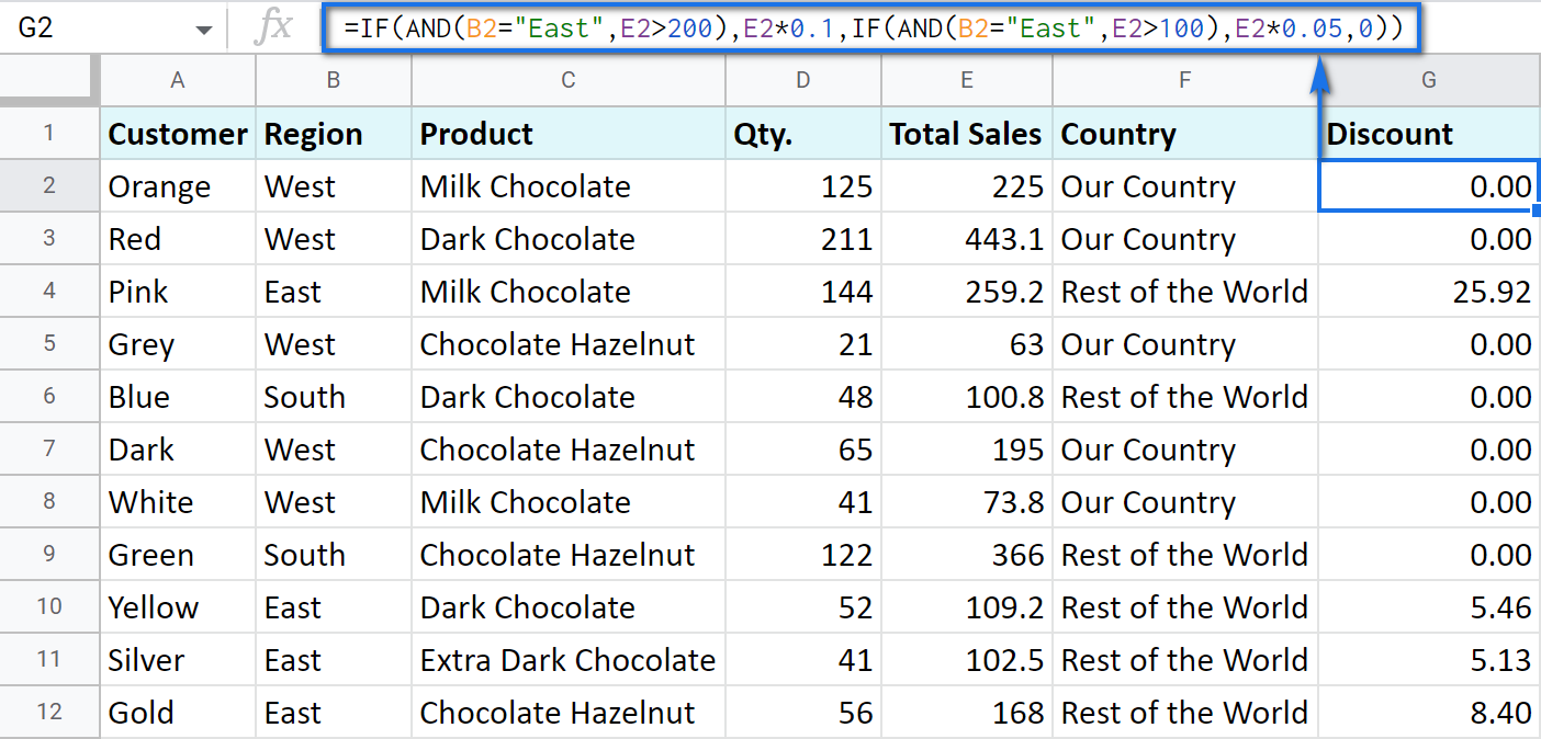
As you can see, the number of discounts has reduced greatly while their amount remains intact.
There's also an easier way to write the above thanks to the IFS function:
- condition1 – (required) is the logical expression you want to test.
- value1 – (required) is the value to return if the condition1 is true.
- and then you just list conditions with their values to return if they are true.
Here's how the above formula will look with IFS:
=IFS(AND(B2="East",E2>200),E2*0.1,AND(B2="East",E2>100),E2*0.05)
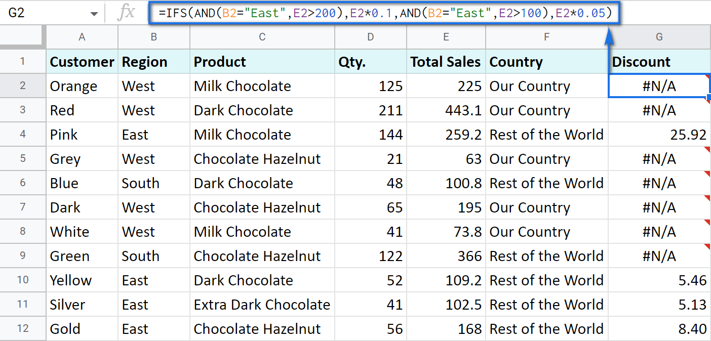
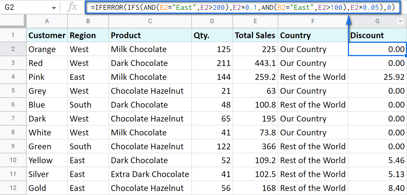
Tip. If there's no true condition, the formula will return the #N/A error. To avoid that, wrap your formula with IFERROR:
=IFERROR(IFS(AND(B2="East",E2>200),E2*0.1,AND(B2="East",E2>100),E2*0.05),0)
SWITCH as an alternative to multiple IFs
There's one more function you may want to consider instead of the nested IF: Google Sheets SWITCH.
It checks if your expression corresponds to a list of cases, one by one. When it does, the function returns a corresponding value.
- expression is any cell reference, or a range of cells, or even an actual math expression, or even a text that you'd like to equal to your cases (or test against the criteria). Required.
- case1 is your first criteria to check the expression against. Required.
- value1 is a record to return if the case1 criterion is the same as your expression. Required.
- case2, value2 repeat as many times as criteria you have to check and values to return. Optional.
- default is also completely optional. Use it to see a specific record if none of the cases is met. I'd recommend using it every time to avoid errors when your expression doesn't meet matches among all the cases.
Here are a couple of examples.
To test your cells against a text, use ranges as an expression:
=ARRAYFORMULA(SWITCH(B2:B69,"West","Our Country","Rest of the World"))
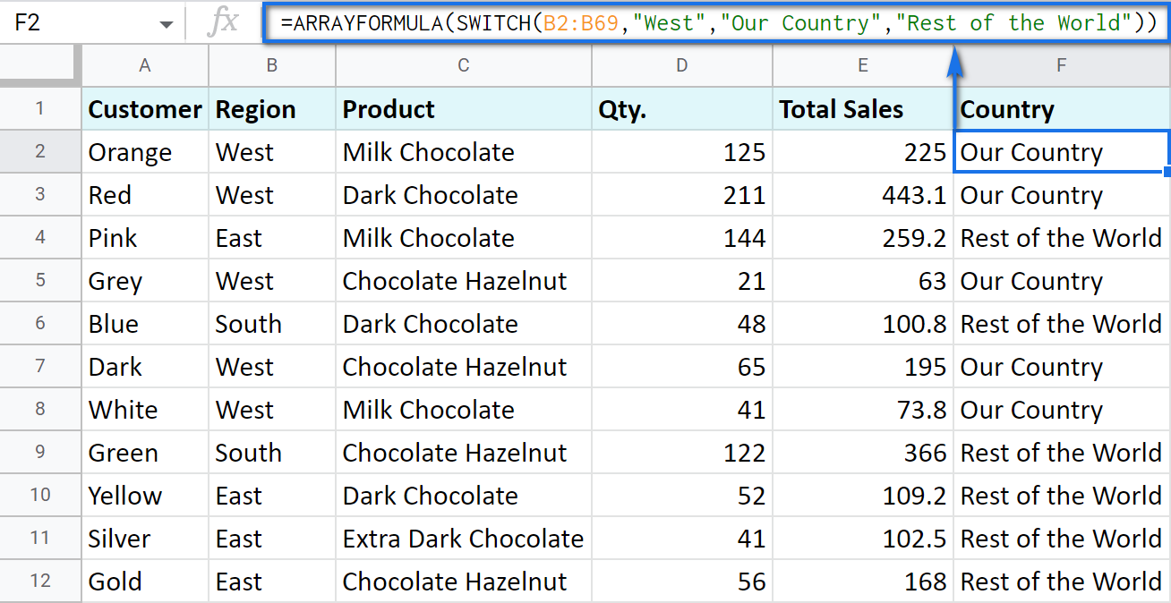
In this formula, SWITCH checks what record is in every cell in column B. If it's West, the formula says Our Country, otherwise, Rest of the World. ArrayFormula makes it possible to process the entire column at once.
To work with calculations, it's better to use a boolean expression:
=SWITCH(TRUE,$E2>200,$E2*0.1,AND($E2<200,$E2>100),$E2*0.05,0)
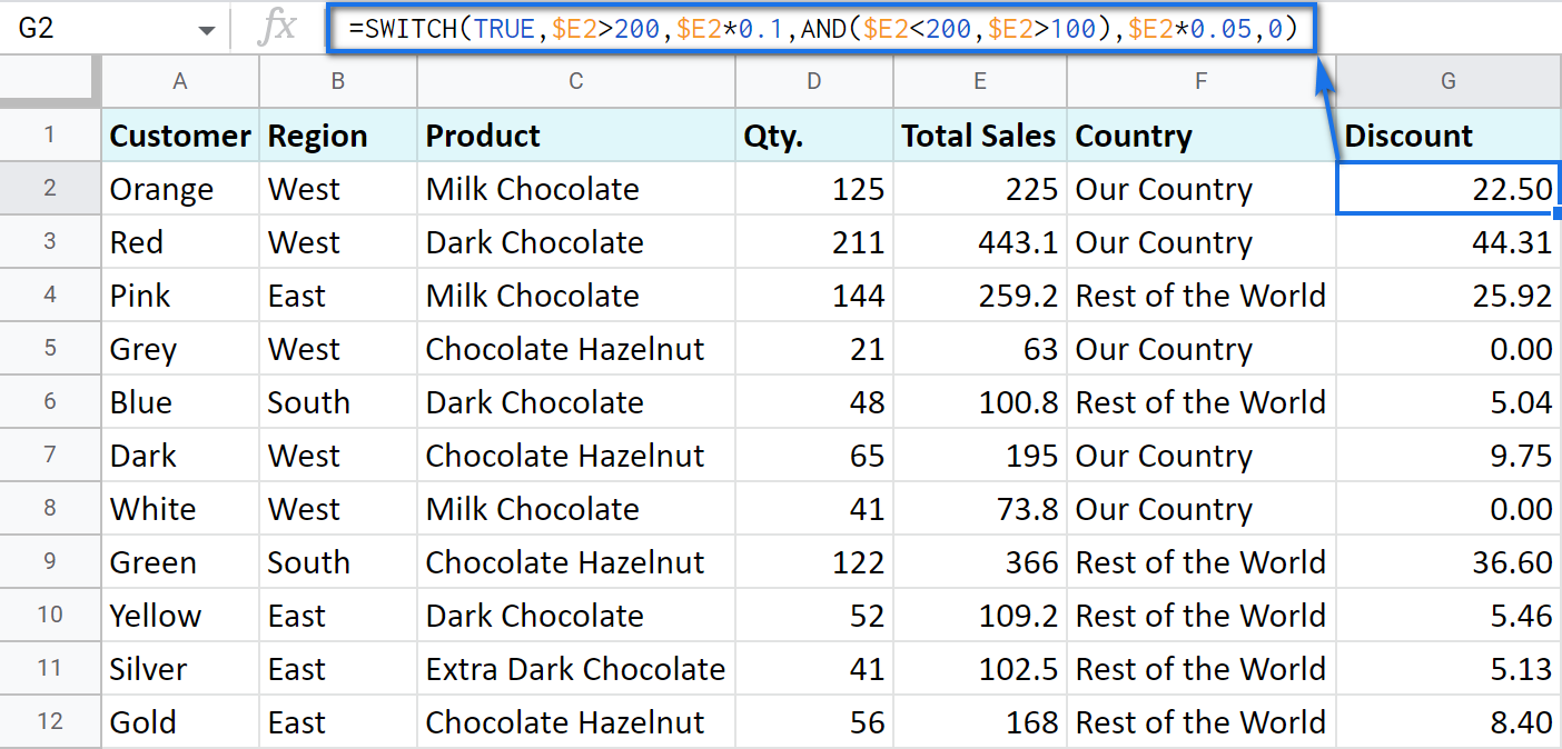
Here SWITCH checks if the result of the equation is TRUE or FALSE. When it's TRUE (like if E2 is really greater than 200), I get a corresponding result. If none of the cases in the list is TRUE (meaning they are FALSE), the formula simply returns 0.
Note. SWITCH doesn't know how to calculate the entire range at once, so no ARRAYFORMULA in this case.
IF statements based on a count
One of the questions we get asked a lot is how to create the IF formula that will return whatever you need if the column contains or doesn't contain a certain record.
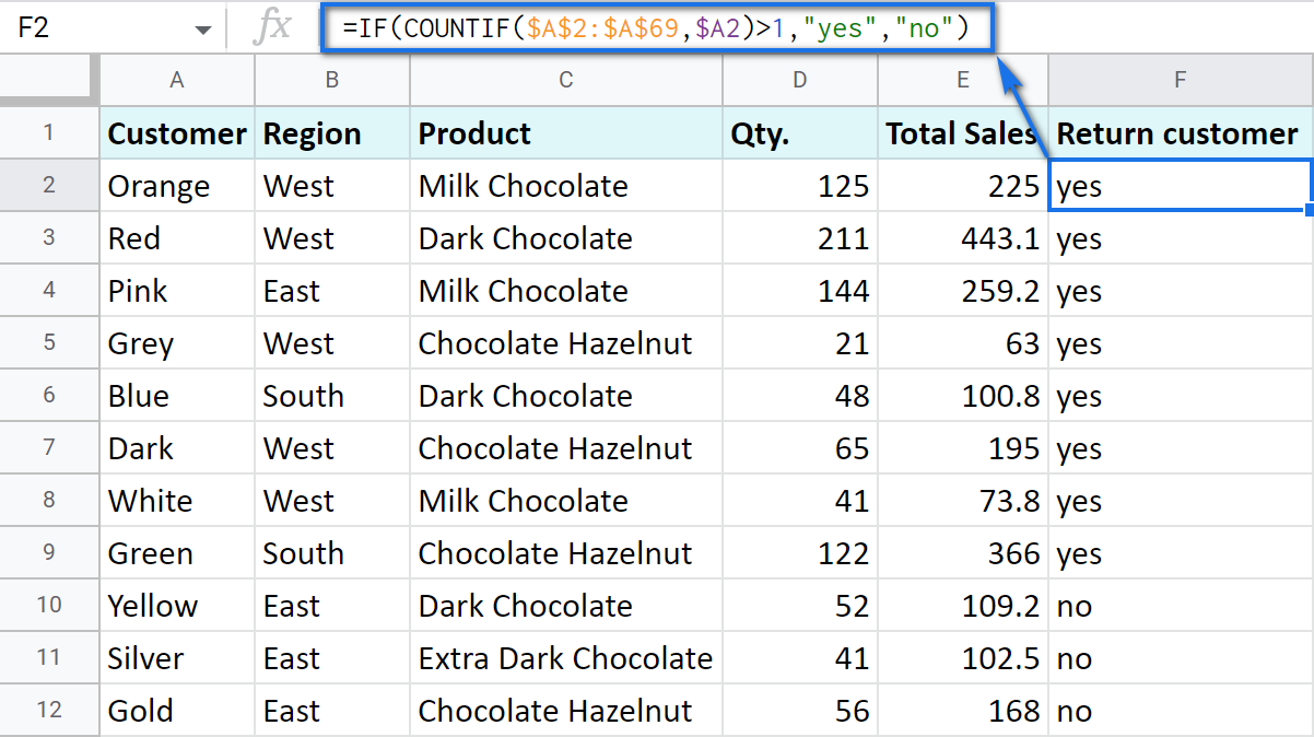
For example, check if a customer's name appears more than once in a list (column A) and put the corresponding word (yes/no) into a cell.
A solution is simpler than you may think. You need to introduce the COUNTIF function to your IF:
=IF(COUNTIF($A$2:$A$69,$A2)>1,"yes","no")
Make Google Sheets build IF formulas for you – IF Formula Builder add-on
If you're tired of keeping track of all those extra characters and proper syntax in formulas, there's another solution available.
IF Formula Builder add-on for Google Sheets offers a visual way of creating IF statements. The tool will handle syntax, extra functions and all required characters for you.
All you need to do is:
- fill blanks with your records one by one. No special treatment for dates, time, etc. Enter them as you always do and the add-on will recognize the data type.
- select required comparison operators from the suggested drop-down lists.
- if needed, add multiple logical expressions in a click: IF OR, IF AND, ELSE IF, THEN IF.
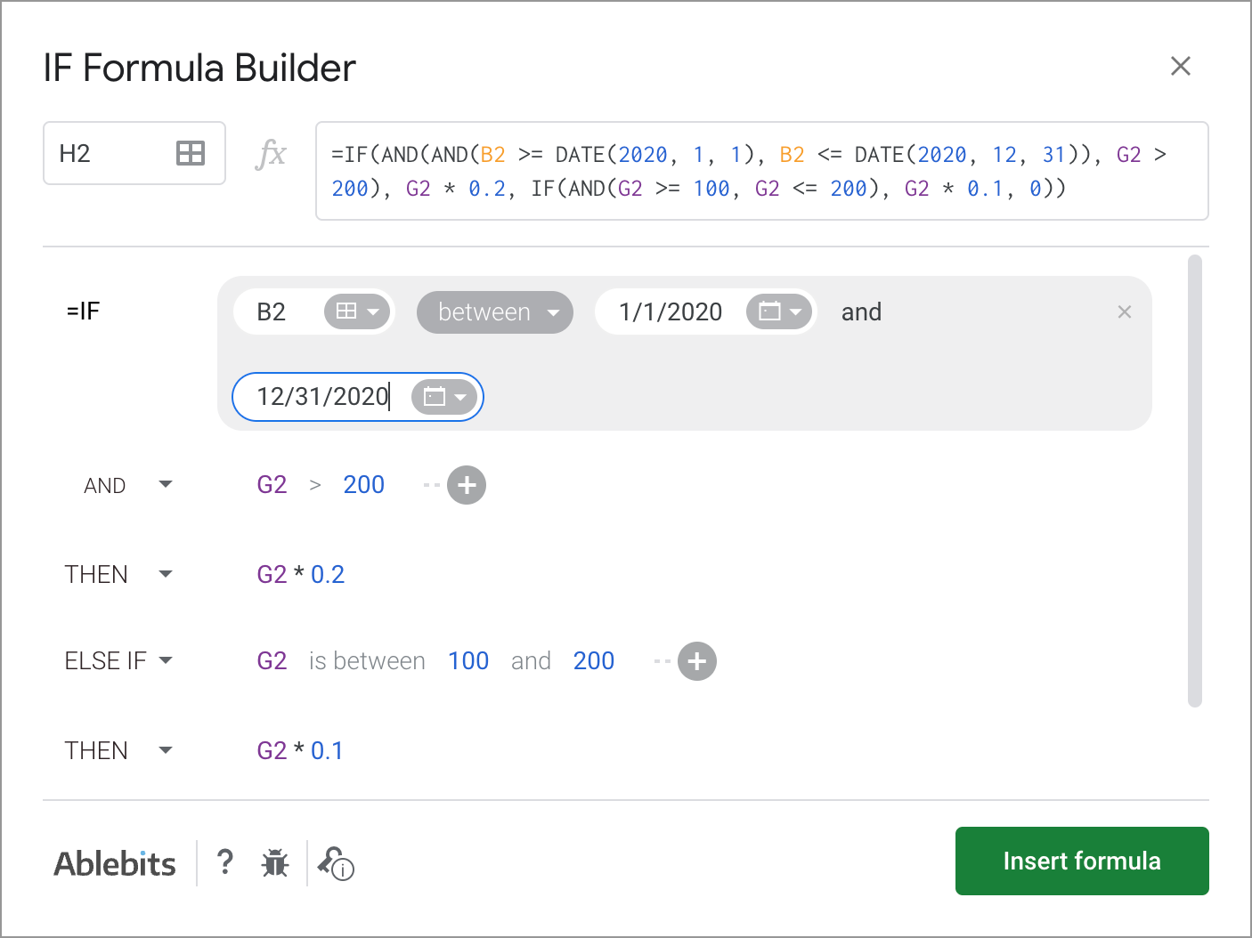
As you can see, each logical expression takes its own line. The same goes for true/false outcomes. This reduces the number of possible confusion over the formula drastically.
As you fill everything out, the formula for use will grow in the preview area at the top of the window. To its left, you can select a cell in your sheet where you'd like to have the formula.
When you're ready, paste the formula into the cell of interest by clicking the Insert formula button at the bottom.
Please visit the online tutorial for IF Formula Builder to see all options described in detail.
I hope that there's no room for any doubt now that the IF function, though a very simple one at first glance, opens the door to many options for data processing in Google Sheets. But if you still have questions, feel free to ask them in the comments section down below – we'll be happy to help!
 by
by
607 comments
MILES RATE TOTAL
34 1.88 $366.22
How do i put a mileage range of numbers like this
miles rate
0 to 5.9 = 1.01
6 to 10.9 = 1.11
11 to 15.9 = 1.25
and so on in to a formula any help would be great.
Hello Patrick,
If I understand your task correctly, here's how you should put that down to the formula (supposing everything starts from A1):
=IF(AND(A2>=0,A2<=5.9),1.01,IF(AND(A2>=6,A2<=10.9),1.11,IF(AND(A2>=11,A2<=15.9),1.25,IF(AND(A2...),1.88,IF...))))
Were you able to get this to work? I tried something similar and am returning an error message.
=IF(AND(D30>749,D301625,D30=2500),$1500)))
Hi Ben,
You miss the comparison operator in your second condition: D301625
Also, I don't see the point of using AND to check whether D30 equals 2500 and is more than 749 at the same time. :) It is either equal to 2500 or not.
If you clarify your conditions, I might be able to help you with the formula.
Thank you so much for this page.
Because of it I was able to figure out how to make text in one column trigger text in another.
Formula
=IF(OR(F2="Planning"),"BLACK",IF(OR(F2="Started"),"RED",IF(OR(F2="Hold"),"BLUE",IF(OR(F2="Complete"),"GREEN"))))
Thank you for your feedback, Laura.
Your formula looks nice :) But there's no need to use OR. It is used to check if at least one of the specified conditions is met, like this: =IF(OR(F2="Planning",F2="Started"),"BLACK",...
Thus, you can get by with the following:
=IF(F2="Planning","BLACK",IF(F2="Started","RED",IF(F2="Hold","BLUE",IF(F2="Complete","GREEN"))))
You can also add one last part - double quotes - to keep cells empty if none of the conditions are met: ...,IF(F2="Complete","GREEN",""))))
So, I want a value to appear based on 2 cells, not one. So like A1 has to be 2 & A2 has to be 4 in order for the value/text to appear. Is there a formula for that?
Of course, there is:
=IF(AND(A1=2,A2=4),"YOUR TEXT","")
I'm looking for a formula to look at a range of cells in a column and look for someone's name. If the name is there, I'd like it to return "Yes"; if it is not there, I'd like it to return "No." I can't quite seem to get it to work! Is there a way to do this?
Alison,
You need to wrap COUNTIF with IF.
Suppose your names are in column A. You can try this formula in B1. Just replace NAME in double-quotes with a name you want to scan for:
=IF(COUNTIF($A$1:$A$20,"NAME")>0,"Yes","No"))
Then just copy the formula down the B column and fill with other names to look up.
update, something like this
=IF(F32=0,"N",IF(F32=,"W")))
Daniel,
to help you out with a formula, I need more details. What should the formula return if cells are less than or equal to -1? And if more than or equal to 1?
Btw, we mentioned nested IF in the last point of this article, please have a look.
trying to create a formula for win loss and neutral using cell=1>, <-1 , 0, for neutral.
If it's more than 1 i want it to show as a "W".
Hi, I have a log for voicemails that includes vm number, client name, date in, date out and who it was forwarded to. What I am trying to do it autopopulate on another tab what calls were sent to whom. so every time I put Missy in the who it was forwarded to column I would like that to fill in a different cell on another sheet with the information from that row. Is this possible??
Hi Missy,
I believe Fran above had a similar question. Please have a look.
If Vlookup doesn't help you, please consider sharing a small sample spreadsheet with us (support@4-bits.com) with your source data and the result you expect to get. I kindly ask you to shorten the tables to 10-20 rows.
I'll look into it and try to help.
How do you make random web-scraped data consistent?
Data values are: 134M , 54B , (230K)
I have a couple functions for making the Millions to Billions consistent.
=if(ISNUMBER(H37), H37, IFERROR( LEFT( H37 , SEARCH( "k" , H37 ) -1) * 1000, IFERROR(LEFT (H37,SEARCH("m", H37 )-1) * 1000000, IFERROR(LEFT (H37,SEARCH("B", H37 )-1) * 1000000000,) )))
and this also :
=left(I37,len(I37)-1)*switch(right(I37,1),"M",1000000,"B",1000000000)
But how do I make a value in parentheses a negative number?
Format changing only, doesn't seem to work in web-scraped data for parentheses.
Robyn,
If we've got your task correctly, the below formula will do the trick:
=IF(LEFT(I37,1)="(",MID(I37,2,LEN(I37)-3)*SWITCH(MID(I37,LEN(I37)-1,1),"K",-1000,"M",-1000000,"B",-1000000000),LEFT(I37,LEN(I37)-1)*SWITCH(RIGHT(I37,1),"K",1000,"M",1000000,"B",1000000000))
Ahh, Thank you Natalia ! :)
Sheet 1 is a master list showing the name of each volunteer organization in Col. A and its assigned trash cleanup location in Col. B. These groups do multiple cleanups each year on random dates. Sheet 2 is where I enter trash cleanup data by date and organization. (The organizations on the master list in Sheet 1 are just a subset of all organizations doing cleanups.) I'd like entry of the name of organization on Sheet 2, say in Col. A, to recognize automatically its corresponding trash cleanup location and enter it in Col. B. I'm unclear on how to set up an IF statement that would match the name of organization with its corresponding trash cleanup location.
Fran,
It is Google Sheets VLOOKUP that you should try rather than IF. Here's a formula based on the task and columns you described:
=ARRAYFORMULA(VLOOKUP(A2:A10,Sheet1!A1:B11,2,0))
A2:A10 is the column with organization names that you enter on Sheet2. You can extend the range based on the number of cells you're going to fill in.
A1:B11 is the range with organization names on Sheet1.
2 - the number of the column with locations on Sheet1.
To learn more about VLOOKUP in Google Sheets, please visit this blog post.
I have linked a form response to a google sheet. I am looking for help as one of the questions is yes or no if someone would like to be added to an email list. I am trying to write an IF formula to have cell $F2 or $F3 is "yes" than cell $C2 or $C3 (the email) moves to another sheet (i.e. Sheet 2, cell $A2 or $A3, etc). Any help would be appreciated.
EF,
try this formula in A2 of Sheet2 and copy down the column:
=IF(Sheet1!$F2="yes",Sheet1!$C2,"")
Or here's an array formula for A2 that helps to avoid copying the formula further:
=ARRAYFORMULA(IF(Sheet2!$F$2:$F$100="yes",Sheet2!$C$2:$C$100,""))
Hi,
I'm looking for some help creating an if-then statement in google docs with conditional formatting. I'd like to populate column E with a 1 or 2 depending on the info in column C. For example, if the name "Cook" is listed in column C then I would need column E to have a 1. Additionally, if column C is Cook or Enright or Sanchez then I would need to mark a 1. TIA!
Hi Lee,
If I understand your task correctly, place the following to E2 assuming your data starts in C2:
=IF(OR(C2="Cook",C2="Enright",C2="Sanchez"),1,2)
As for conditional formatting, it lets you color cells based on conditions. You can learn more about it in this blog post.
Thank you so much! I had the first part correct and appreciate your help! You're awesome
my formula is =IF(C2="Joe Bloggs","Maddie Bloggs","Annie Bloggs") but I want it also be the case if C2=Katy Bloggs and if C2=Rachel Bloggs. How would that look please?
Annie,
try this one:
=IF(OR(C2="Joe Bloggs",C2="Katy Bloggs",C2="Rachel Bloggs"),"Maddie Bloggs","Annie Bloggs")
Hi there, I am attempting to create a formula to lengthen the text imputed. ie: dpst = DPST PENDING(c), under conditional format rules, with highlighting & bold font.. I have custom fomula selecte w/ =if (L2="dpst"," "DPST PENDING") apply to range K2:M2.
I also in the same sheet am trying to create if "conf" is payment type(F), $0.00 balance (O) is due, if Cash, crcd, chk is used, Subtotal (m) - amt pd (N) is balance due (O).
I have came up w/ =ifs(F4="conf",0,F4="cash","crcd","chk",M4-N4).
But nothing is working. Please help!! Much appreciated!!
Hi Susan,
I'm sorry, your conditions for the second formula are quite confusing.
For us to understand your case and check the formulas, please share your sample spreadsheet with us (support@4-bits.com) with your data and the result you expect to get. I kindly ask you to shorten the tables to 10-20 rows.
Since we keep that email for file sharing only, once you share the file, please confirm by replying to my comment here.
Thank you.
I want to make a cell time and date stamp if another cell has text. For example, I am having employees enter in marketing information and I want Google Sheets to tell me exactly when they entered in that specific data point. Something like "If cell E2 has text, then cell G2 get's a time and date stamp."
I thought I might be able to do this with conditional formatting but that is not the case. I'm looking for the easiest fix here with the least amount of code.
Jeff,
The only function that would return you the date time stamp is NOW. However, the function is volatile - it recalculates itself in all cells each time anything is edited in the sheet. Thus, the standard formula is not an option here, I'm afraid. You need to use scripts to solve the task.
You may try to find the solution here - an overview of Google Apps Script with a lot of helpful content and links:
https://developers.google.com/apps-script/overview
Sorry I'm not able to assist you better at the moment.
What is wrong with this IF statement, "=if(=and(B2 - C2 0) "Close Democrat", =if(=and(B2 - C2 5), "Moderate Democrat", =if(b2 - c2 > 7, "Extreme Democrat", =if(=and(B2 - C2 = -5), "Close Republican", =if(=and(B2 - c2 = -10), "Moderate Republican", =if(B2-C2 <= -10, "Extreme Republican"))))))"
The error message reads, "Formula Parse Error". The purpose of this IF statement is to check certain percentage differences and give different responses based on them.
Mark,
You have obsolete equal signs before each IF and AND. Also, the arguments for AND are written incorrectly. Your formula should look like this:
=IF(AND(B2=0,C2=0),"Close Democrat",IF(AND(B2=5,C2=5),"Moderate Democrat",IF... so on
Please look through examples above to learn more about the IF formula.
I have a Google Sheet that has multiple tabs.
If "Head of Household" is entered in Column E on Tab 1, then I want it to bring over the information entered in Column C & D to Tab 2 Columns C & D.
I also do not want any blanks, so I want Tab 2 to only be Head of Household names listed on Tab 1.
William,
It looks like VLOOKUP is the function for your task. This is the function one should use when searching for value in one column and pulling the corresponding info from other columns.
Please help. I'm trying to write an if/then formula based on a count. Count the number of cells in a given row range (G1:Z1) with the text 'Completed' then multiple the number by 3.
Ashley,
Please have a look at the COUNTIF function. It lets you count cells based on your criterion.
If the result for Thu, Aug 22, 2019 (1262) was bigger than Wed, Aug 21, 2019 (1124) to highlight the result in a custom colour or if the result is worse - highlight the result in another custom colour.
Thank you for another explanation, Nikola.
It's a pity the way offered before didn't work as you need.
I'm passing your task to the same tech specialist - hope he'll be able to help!
Nikola,
Please try these formulas in your conditional formatting:
for when yesterday is > than the day before
=AND($A1=TODAY()-1,OFFSET($B1,-1,0)<$B1)
and for when yesterday is < than the day before
=AND($A1=TODAY()-1,OFFSET($B1,-1,0)>$B1)
Hello Natalia,
Thank you for your response!
Take a look at this example of my sheet:
Column A Column B
Mon, Aug 12, 2019 1695
Tue, Aug 13, 2019 1463
Wed, Aug 14, 2019 1395
Thu, Aug 15, 2019 1325
Fri, Aug 16, 2019 1267
Sat, Aug 17, 2019 1396
Sun, Aug 18, 2019 1100
Mon, Aug 19, 2019 1510
Tue, Aug 20, 2019 1238
Wed, Aug 21, 2019 1124
Thu, Aug 22, 2019 1262
I would like to use conditional formatting to highlight when -> my yesterday result was better/worse than the day before.
If yesterday is < than the day before, show RED
Hello, some help here?
Hello Nikola,
Your task is not an easy one, and I've forwarded it to our tech team. As soon as I have a solution, I'll reply right away.
Sorry for the inconvenience.
Thank you!
Looking for your response.
Nikola,
Here's what we've got for now:
1) =AND($A1<$A2,$A1=$A2-1,$B1>$B2)
This formula makes sure that the date in A2 is greater than in A1 but the corresponding number is A2 is less than in A1. If your data to compare starts in A1, skip it and apply the formula to your table starting from A2.
2) =AND($A1<$A2,$A1=$A2-1,$B1>$B2)
This one does the same but also checks if the difference between dates is 1 day only.
If these are not exactly what you need, please share a sample spreadsheet with us (support@4-bits.com) with a short example table and the result you expect to get. We don’t monitor the Inbox of that email though, so please confirm by replying here once you share the file. Thank you.