This tutorial shows how to use INDEX and MATCH in Excel and how it is better than VLOOKUP.
In a couple of recent articles, we made a good effort to explain the basics of VLOOKUP function to beginners and provide more complex VLOOKUP formula examples to power users. And now, I will try if not to talk you out of using VLOOKUP, then at least show you an alternative way to do a vertical lookup in Excel.
"What do I need that for?" you may wonder. Because VLOOKUP has numerous limitations that can prevent you from getting the desired result in many situations. On the other hand, the INDEX MATCH combination is more flexible and has many awesome features that make it superior to VLOOKUP in many respects.

Excel INDEX and MATCH functions - the basics
Since the aim of this tutorial is to demonstrate an alternative way to do a vlookup in Excel by using a combination of INDEX and MATCH functions, we won't dwell much on their syntax and uses. We will cover only the minimum necessary for understanding the general idea and then take an in-depth look at formula examples that reveal all the advantages of using INDEX MATCH instead of VLOOKUP.
INDEX function - syntax and usage
The Excel INDEX function returns a value in an array based on the row and column numbers you specify. The syntax of the INDEX function is straightforward:
Here is a very simple explanation of each parameter:
- array - a range of cells that you want to return a value from.
- row_num - the row number in array from which you want to return a value. If omitted, the column_num is required.
- column_num - the column number in array from which you want to return a value. If omitted, row_num is required.
For more information, please see Excel INDEX function.
And here is an example of the INDEX formula in its simplest form:
=INDEX(A1:C10,2,3)
The formula searches in cells A1 through C10 and returns a value of the cell in the 2nd row and the 3rd column, i.e. cell C2.
Very easy, right? However, when working with real data you would hardly ever know which row and column you want, that's where the MATCH function comes in handy.
MATCH function - syntax and usage
The Excel MATCH function searches for a lookup value in a range of cells and returns the relative position of that value in the range.
The syntax of the MATCH function is as follows:
- lookup_value - the number or text value you are looking for.
- lookup_array - a range of cells being searched.
- match_type - specifies whether to return an exact match or the nearest match:
- 1 or omitted (default) - approximate match (next smaller).
- 0 - exact match. In the INDEX / MATCH combination, you almost always need an exact match, so you set the third argument of your MATCH function to 0.
- -1 - approximate match (next larger).
For example, if the range B1:B3 contains the values "New-York", "Paris", "London", the below formula returns the number 3, because "London" is the third entry in the range:
=MATCH("London",B1:B3,0)
For more information, please see Excel MATCH function.
At first sight, the usefulness of the MATCH function may seem questionable. Who cares about the position of a value in a range? What we do want to know is the value itself.
Let me remind you that the relative position of the lookup value (i.e. row and column numbers) is exactly what you need to supply to the row_num and column_num arguments of the INDEX function. As you remember, Excel INDEX can find the value at the juncture of a given row and column, but it cannot determine which exactly row and column you want.
How to use INDEX MATCH function in Excel
Now that you know the basics, I believe it has already started making sense how MATCH and INDEX work together. In a nutshell, INDEX finds the lookup value by column and row numbers, and MATCH provides those numbers. That's it!
For vertical lookup, you use the MATCH function only to determine the row number and supply the column range directly to INDEX:
Still having difficulties to figure that out? It might be easier to understand from an example. Suppose you have a list of national capitals and their population:

To find the population of a certain capital, say the capital of Japan, use the following INDEX MATCH formula:
=INDEX(C2:C10, MATCH("Japan", A2:A10, 0))
Now, let's analyze what each component of this formula actually does:
- The MATCH function searches for the lookup value "Japan" in the range A2:A10, and returns the number 3, because "Japan" is third in the lookup array.
- The row number goes directly to the row_num argument of INDEX instructing it to return a value from that row.
So, the above formula turns into a simple INDEX(C2:C,3) that says to search in cells C2 through C10 and pull the value from the 3rd cell in that range, i.e. C4 because we start counting from the second row.
Don't want to hardcode the city in the formula? Input it in some cell, say F1, supply the cell reference to MATCH, and you will get a dynamic lookup formula:
=INDEX(C2:C10, MATCH(F1,A2:A10,0))
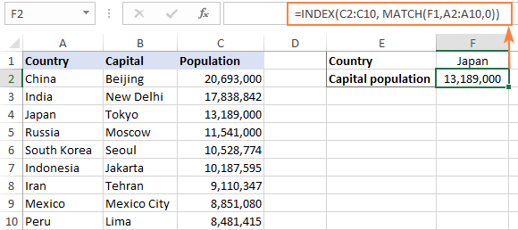
Important note! The number of rows in the array argument of INDEX should match the number of rows in the lookup_array argument of MATCH, otherwise the formula will produce an incorrect result.
Wait, wait… why don't we simply use the following Vlookup formula? What's the point in wasting time trying to figure out the arcane twists of Excel MATCH INDEX?
=VLOOKUP(F1, A2:C10, 3, FALSE)
In this case, no point at all :) This simple example is for demonstration purposes only, so that you get a feel of how the INDEX and MATCH functions work together. Other examples that follow below will show you the real power of this combination that easily copes with many complex scenarios when VLOOKUP stumbles.
Tips:
- In Excel 365 and Excel 2021, you can use a more modern INDEX XMATCH formula.
- For Google Sheets, see formula examples with INDEX MATCH in this article.
INDEX MATCH vs. VLOOKUP
When deciding which function to use for vertical lookups, most Excel gurus agree that INDEX MATCH is far better than VLOOKUP. However, many people still stay with VLOOKUP, firstly, because it's simpler and, secondly, because they do not fully understand all benefits of using the INDEX MATCH formula in Excel. Without such understanding no one is willing to invest their time to learn a more complex syntax.
Below, I will point out the key advantages of MATCH INDEX over VLOOKUP, and you decide whether it's a worthy addition to your Excel arsenal.
4 main reasons to use INDEX MATCH instead of VLOOKUP
- Right to left lookup. As any educated user knows, VLOOKUP cannot look to its left, meaning your lookup value should always reside in the leftmost column of the table. INDEX MATCH can do left lookup with ease! The following example shows it in action: How to Vlookup a value to the left in Excel.
- Insert or delete columns safely. VLOOKUP formulas get broken or delivers incorrect results when a new column is deleted from or added to a lookup table because VLOOKUP's syntax requires specifying the index number of the column you want to pull the data from. Naturally, when you add or delete columns, the index number changes.
With INDEX MATCH, you specify the return column range, not an index number. As the result, you are free to insert and remove as many columns as you want without worrying about updating every associated formula.
- No limit for a lookup value's size. When using the VLOOKUP function, the total length of your lookup criteria cannot exceed 255 characters, otherwise you will end up having the #VALUE! error. So, if your dataset contains long strings, INDEX MATCH is the only working solution.
- Higher processing speed. If your tables are relatively small, there will hardly be any significant difference in Excel performance. But if your worksheets contain hundreds or thousands of rows, and consequently hundreds or thousands of formulas, MATCH INDEX will work much faster than VLOOKUP because Excel will have to process only the lookup and return columns rather than the entire table array.
VLOOKUP's impact on Excel's performance may be especially noticeable if your workbook contains complex array formulas like VLOOKUP and SUM. The point is that checking each value in the array requires a separate call of the VLOOKUP function. So, the more values your array contains and the more array formulas you have in a workbook, the slower Excel performs.
To discover the nuanced differences between INDEX MATCH and XLOOKUP, explore the in-depth analysis in this guide: Excel XLOOKUP vs INDEX MATCH.
Excel INDEX MATCH - formula examples
Knowing the reasons to learn the MATCH INDEX function, let's get to the most interesting part and see how you can apply the theoretical knowledge in practice.
INDEX MATCH formula to look up from right to left
As already mentioned, VLOOKUP cannot look at its left. So, unless your lookup values are is the leftmost column, there's no chance that a Vlookup formula will bring you the result you want. The INDEX MATCH function in Excel is more versatile and does not really care where the lookup and return columns are located.
For this example, we will add the Rank column to the left of our sample table and try to figure out how the Russian capital, Moscow, ranks in terms of population.
With the lookup value in G1, use the following formula to search in C2:C10 and return a corresponding value from A2:A10:
=INDEX(A2:A10,MATCH(G1,C2:C10,0))
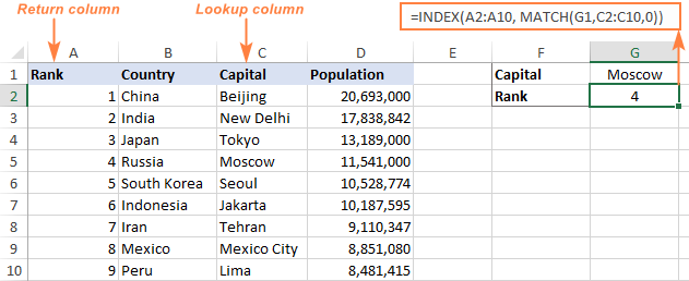
Tip. If you plan to use your INDEX MATCH formula for more than one cell, be sure to lock both ranges with absolute cell references (like $A$2:$A$10 and $C$2:4C$10) so they won't get distorted when copying the formula.
INDEX MATCH MATCH to search in rows and columns
In the above examples, we used INDEX MATCH as the replacement for classic VLOOKUP to return a value from a predefined one-column range. But what if you need to look up in multiple rows and columns? In other words, what if you want to perform the so-called matrix or two-way lookup?
This may sound tricky, but the formula is very similar to the basic Excel INDEX MATCH function, with just one difference. Guess what?
Simply, use two MATCH functions – one to get a row number and the other to get a column number. And I congratulate those of you who have guessed right :)
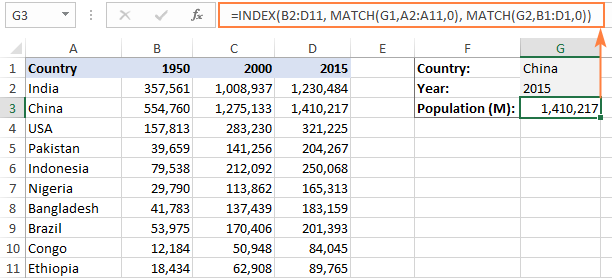
And now, please take a look at the below table and let's build an INDEX MATCH MATCH formula to find the population (in millions) in a given country for a given year.
With the target country in G1 (vlookup value) and the target year in G2 (hlookup value), the formula takes this shape:
=INDEX(B2:D11, MATCH(G1,A2:A11,0), MATCH(G2,B1:D1,0))
How this formula works
Whenever you need to understand a complex Excel formula, break it down into smaller parts and see what each individual function does:
MATCH(G1,A2:A11,0) – searches through A2:A11 for the value in cell G1 ("China") and returns its position, which is 2.
MATCH(G2,B1:D1,0)) – searches through B1:D1 to get the position of the value in cell G2 ("2015"), which is 3.
The above row and column numbers go to the corresponding arguments of the INDEX function:
INDEX(B2:D11, 2, 3)
As the result, you get a value at the intersection of the 2nd row and 3rd column in the range B2:D11, which is the value in cell D3. Easy? Yep!
Excel INDEX MATCH to look up multiple criteria
If you had a chance to read our Excel VLOOKUP tutorial, you have probably already tested a formula to Vlookup with multiple criteria. However, a significant limitation of that approach is the necessity to add a helper column. The good news is that Excel's INDEX MATCH function can look up with two or more criteria too, without modifying or restructuring your source data!
Here's the generic INDEX MATCH formula with multiple criteria:
Note. This is an array formula that must be completed with the Ctrl + Shift + Enter shortcut.
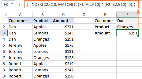
In the sample table below, supposing you want to find the amount based on 2 criteria, Customer and Product.
The following INDEX MATCH formula works a treat:
=INDEX(C2:C10, MATCH(1, (F1=A2:A10) * (F2=B2:B10), 0))
Where C2:C10 is the range to return a value from, F1 is criteria1, A2:A10 is the range to compare against criteria1, F2 is criteria 2, and B2:B10 is the range to compare against criteria2.
Remember to enter the formula correctly by pressing Ctrl + Shift + Enter, and Excel will automatically enclose it curly brackets as shown in the screenshot:
If you'd rather not use array formulas in your worksheets, add one more INDEX function to the formula and complete it with a usual Enter hit:

How these formulas work
The formulas use the same approach as the basic INDEX MATCH function that looks through a single column. To evaluate multiple criteria, you create two or more arrays of TRUE and FALSE values that represent matches and non-matches for each individual criterion, and then multiply the corresponding elements of these arrays. The multiplication operation converts TRUE and FALSE into 1 and 0, respectively, and produces an array where 1's correspond to rows that match all the criteria. The MATCH function with a lookup value of 1 finds the first "1" in the array and passes its position to INDEX, which returns a value in this row from the specified column.
The non-array formula relies on the ability of the INDEX function to handle arrays natively. The second INDEX is configured with 0 row_num so that it will pass the entire column array to MATCH.
That is a high-level explanation of the formula's logic. For full details, please see Excel INDEX MATCH with multiple criteria.
Excel INDEX MATCH with AVERAGE, MAX, MIN
Microsoft Excel has special functions to find a minimum, maximum and average value in a range. But what if you need to get a value from another cell that is associated with those values? In this case, use the MAX, MIN or AVERAGE function together with INDEX MATCH.
INDEX MATCH with MAX
To find the largest value in column D and return a value from column C in the same row, use this formula:
=INDEX(C2:C10, MATCH(MAX(D2:D10), D2:D10, 0))
INDEX MATCH with MIN
To locate the smallest value in column D and pull an associated value from column C, use this one:
=INDEX(C2:C10, MATCH(MIN(D2:D10), D2:D10, 0))
INDEX MATCH with AVERAGE
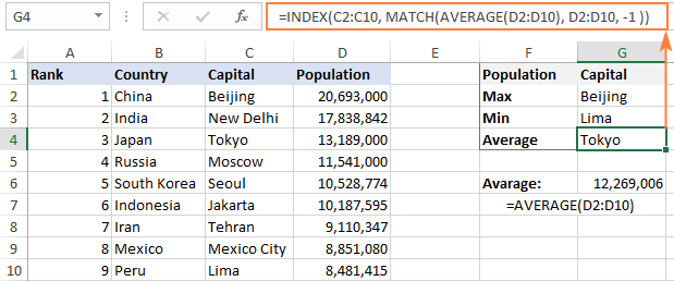
To work out the value closest to the average in D2:D10 and get a corresponding value from column C, this is the formula to use:
=INDEX(C2:C10, MATCH(AVERAGE(D2:D10), D2:D10, -1 ))
Depending on how your data is organized, supply either 1 or -1 to the third argument (match_type) of the MATCH function:
- If your lookup column (column D in our case) is sorted ascending, put 1. The formula will calculate the largest value that is less than or equal to the average value.
- If your lookup column is sorted descending, enter -1. The formula will compute the smallest value that is greater than or equal to the average value.
- If your lookup array contains a value exactly equal to the average, you can enter 0 for exact match. No sorting is required.
In our example, the populations in column D are sorted in descending order, so we use -1 for match type. As the result, we get "Tokyo" since its population (13,189,000) is the closest match that is greater than average (12,269,006).
You may be curious to know that VLOOKUP can perform such calculations too, but as an array formula: VLOOKUP with AVERAGE, MAX, MIN.
Using INDEX MATCH with IFNA / IFERROR
As you have probably noticed, if an INDEX MATCH formula in Excel cannot find a lookup value, it produces an #N/A error. If you wish to replace the standard error notation with something more meaningful, wrap your INDEX MATCH formula in the IFNA function. For example:
=IFNA(INDEX(C2:C10, MATCH(F1,A2:A10,0)), "No match is found")
And now, if someone inputs a lookup table that does not exist in the lookup range, the formula will explicitly inform the user that no match is found:

If you'd like to catch all errors, not only #N/A, use the IFERROR function instead of IFNA:
=IFERROR(INDEX(C2:C10, MATCH(F1,A2:A10,0)), "Oops, something went wrong!")
Please keep in mind that in many situations it might be unwise to disguise all errors because they alert you about possible faults in your formula.
That's how to use INDEX and MATCH in Excel. I hope our formula examples will prove helpful for you and look forward to seeing you on our blog next week!
Practice workbook for download
Excel INDEX MATCH examples (.xlsx file)
 by
by
614 comments
Hello Svetlana
I am started to use Index Match function and I tried your article/suggestion very useful.
I have now looking at using Index Match with multiple criteria and I followed the example. I have noted that in this case one of the advantages wrt vlookup value use is lost, basically I can not longer insert or delete column in the lookup table. Can you please confirm that? is there 1 alternative can be use that overrides this problem
Thanks
S
Hi. An excellent article on the use of INDEX MATCH, thank you. I have added the error handler (IFERROR) but previously with VLOOKUP I could also check to see if the resulting value was blank, and leave it blank in the cell. The data type in my cell is DATE, and if the answer is 0, it formats this as a date which is a pain.
My old formula is: =IFERROR(IF(ISBLANK(VLOOKUP(A1,Endorsements!A2:L33,5,FALSE)),"",VLOOKUP(A1,Endorsements!A2:L33,5,FALSE)),"")
I now have =IFERROR(INDEX(Endorsements!$E:$E,MATCH(A1,Endorsements!$A:$A,0)),"") which works great unless the item found is a 0, in which case the cell then shows 00 Jan 00.
Hope you can assist, this has been baffling me for many hours!
Thank you
Thanks a lot to post a very useful topic which can minimize our work at a great extent.
HELLO
i have a master list of items and New items codes . and another list of secondary list of items which have old codes .
I need to find out the common item description and replace the old item codes with the new codes.
thanks
Hi Svetlana! I have a spreadsheet with NFL stats and player rankings for all teams. My quarterback rankings are on Sheet 1 and wide receivers on Sheet 2.
I am trying to add the ranking of a quarter back with the ranking of a wide receiver for the same team to return a value for the wide receiver.
Example: wide receiver Joe Smith plays for team X and is ranked #5, his quarter back John Doe is ranked 6 = Joe Smith's value of 11.
Here is one formula that I've tried unsuccessfully so far : =IF(MATCH(C2:C51,Sheet2!C2:C39,0),A2:A51+Sheet2!A2:A39). Thank you for any assistance provided.
Hi every one.
Whats the simple way to do this
* If the DATE entered in "X" sheet goes to same date cell i.e if entered 10th then its goes to 10th Row of "Y"sheet".
Thanking you in advance for your kind support
I am new to the Vlookup function, I feel I have a good grasp of it but one of my basic lookups is not working correctly. Ifyou look at test sheet, cell c24. The value is not returning correctly, there seems to be some math occurning and I cant figure out where it is. Any assistance?
C24 - =IFERROR(VLOOKUP(A24,Sheet1!A2:B23,2),0)
I was trying to post the xls but don't see an attachment option.
Hello,
I'm wondering if anyone can help me.
I am trying to create an organiser for my other half for university. Column C10,313 contains the date with column D10,313 Containing work set and a few other columns ToDo, Exams, Notes etc.
I am trying to create a formula with INDEX MATCH to create a new table with a column for 'Work to be completed' and the date set sequentially so when the organiser is being used you don't have to use any filtering functions to search the organiser. I want to keep the interface as simple as possible so you just have to fill in the 'work set' next to the date and it auto populates the concise list of 'Work to be completed' with corresponding date...
Any one know how I can go about this? It would be much appreciated.
Cheers,
Lewis
Hi
I have downloaded Microsoft Templates file called "Sales invoice tracker" which has 4 key tabs which enables me to enter Customer details, Invoice details, Invoice summary and has a Invoice template tab. The file works great for recording all client information, client sales and creates the invoice via a dropdown list named (rngInvoice in the formula below) and referenced by the chosen job number in the "invoice" template. The formula has work fine until the ROW(1:1)) reaches ROW(13:13)) down the invoice page, i have reviewed the formula and for the life of me i cannot understand how this part of ROW works
=IFERROR(INDEX(InvoiceDetails,SMALL(IF(InvoiceDetails[Invoice '#]=rngInvoice,ROW(InvoiceDetails)-ROW(InvoiceDetails[#Headers])), ROW(1:1)), MATCH($B$13, InvoiceDetails[#Headers], 0)),"")
I have recreated a similar document but i am struggling with capturing and transferring data of multiple columns and rows via a single Job number column
All i would like to do is select a Job number on the dropdown list on the "invoice" template and have the data from the "invoice details" with multiple columns and rows to be copied into multiple columns and rows on the invoice
Please help
Hi
I have a file with 2 tabs, the first one has the customers name and the quantity that they ordered by style and on the second tab I also have the customer name and the style that they forecasted, I want to match the customer name and the style of the first tab with the second tab and return the value of the cell with the forecast quantity. I'm using the below formula, but it is not working
=IFERROR(INDEX(Sheet2!$1:$65536,MATCH($A4:$B4,Sheet2!$C:$D,0),MATCH(D$3,Sheet2!$1:$1,0),1),0)
Hi
Anyone can help me to change this vlookup function to index mach?
=IFERROR(VLOOKUP("*"&G:G&"*",'ADV. & LOAN'!B:D,2,FALSE),"")
To be clearer in my last comment, "STREET" is the same as "Street", but is not the same as "Street.". (In my case, comparing addresses, " Lake St." is not the same as "LAKE ST" without the abbreviating period.)
By the way, I did some experiments and even if you pick exact match (0), it is still case insensitive when you try to match.
STREET is the same as Street.
(Now if I could get a "fuzzy" match so that Road would match RD, wow!)
could you please help me out on this scenario.
SCENARIO
IF cell D3 AND range F3:AJ3 ISBLANK(), THEN C3 =""
IF cell D3 OR range F3:AJ3 is NOT BLANK , THEN MATCH values of cell D3 with Range F2:AJ2, whichever is MAX should show in cell C3.
=IF(ISNA(OR(COUNTA(F3:AJ3)=0,(MAX(LOOKUP(2,1/(F3:AJ3""),$F$2:$AJ$2)<D3)))),IF(D3="","",D3),LOOKUP(2,1/(F3:AJ3""),$F$2:$AJ$2))
Hi Svetlana,
Can you kindly show us how we use this function between two worksheet but the excel book is same.I have tired it but i did not completely successful.
Hi Svetlana,
I'm dealing with a software that uses excel functionnalities, but can't support array functions. Do you know an alternate way of doing what an array formula does?
Thanks,
Félix
Sorry the table collapsed!
……A………………………B………………………C………………………………D……………………………………………………E
Alpha………………1234………………Here……………East Here…………………………………………2054
East Here……2054…………………………………….Here…………………………………………………….1223
Golf…………………4657…………………………………….North Here………………………………………2212
Here…………………1223…………………………………….The North Here of Little Westerly…1235
Juliet……………7511…………………………………….West Here…………………………………………5589
North Here…2212
Siera………………4651
The North Here of Little Westerly……….1235
West Here…………………………………………..5589
Thank you
Svetlana
I have a large spreadsheet that contains a lot of information about thousands of locations. Each location has a unique 4 digit index number and a name. The name may not be unique but may be used in different locations such as North Here, South Here, East Here or “The North here of Little Easterly”. Some people know the location by the number and some people know the location by simply, in this case, “Here”. A simple lookup table can be used in the first instance for the unique number but what code must I use so that by entering the name, “Here” in a field, the code placed in stacked fields (say 6, one above the other) will pull up all results where the name “Here” is contained in the text in the field and report the unique location number in the adjacent field:
A B C D E
Alpha 1234 Here East Here 2054
East Here 2054 Here 1223
Golf 4657 North Here 2212
Here 1223 The North Here of Little Westerly 1235
Juliet 7511 West Here 5589
North Here 2212
Siera 4651
The North Here
of Little Westerly 1235
West Here 5589
Thank you
Svetlana
I have a large spreadsheet that contains a lot of information about many locations.
Each location has a unique 4 digit index number and a name. The name may not be unique but may be used in different locations such as North Here, South Here, East Here or “The North here of Little Easterly”. Some people know the location by the number and some people know the location by simply, in this case, “Here”. A simple lookup table can be used in the first instance for the unique number but what code must I use so that by entering the name, “Here” in a field, the code placed in stacked fields (say 6, one above the other) will pull up all results where the name “Here” is contained in the text in the field and report the unique location number in the adjacent field:
A B C D E
Alpha 1234 Here East Here 2054
East Here 2054 Here 1223
Golf 4657 North Here 2212
Here 1223 The North Here of Little Westerly 1235
Juliet 7511 West Here 5589
North Here 2212
Siera 4651
The North Here
of Little Westerly 1235
West Here 5589
Thank you
Sir, Still I am waiting for your positive reply.
Binoy