In this tutorial, you will find a number of formula examples that demonstrate the most efficient uses of INDEX in Excel.
Of all Excel functions whose power is often underestimated and underutilized, INDEX would definitely rank somewhere in the top 10. In the meantime, this function is smart, supple and versatile.
So, what is the INDEX function in Excel? Essentially, an INDEX formula returns a cell reference from within a given array or range. In other words, you use INDEX when you know (or can calculate) the position of an element in a range and you want to get the actual value of that element.
This may sound a bit trivial, but once you realize the real potential of the INDEX function, it could make crucial changes to the way you calculate, analyze and present data in your worksheets.
Excel INDEX function - syntax and basic uses
There are two versions of the INDEX function in Excel - array form and reference form. Both forms can be used in all versions of Microsoft Excel 365 - 2003.
INDEX array form
The INDEX array form returns the value of a certain element in a range or array based on the row and column numbers you specify.
- array - is a range of cells, named range, or table.
- row_num - is the row number in the array from which to return a value. If row_num is omitted, column_num is required.
- column_num - is the column number from which to return a value. If column_num is omitted, row_num is required.
For example, the formula =INDEX(A1:D6, 4, 3) returns the value at the intersection of the 4th row and 3rd column in range A1:D6, which is the value in cell C4.
To get an idea of how the INDEX formula works on real data, please have a look at the following example:
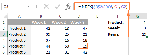
Instead of entering the row and column numbers in the formula, you can supply the cell references to get a more universal formula: =INDEX($B$2:$D$6, G2, G1)
So, this INDEX formula returns the number of items exactly at the intersection of the product number specified in G2 (row_num) and week number entered in cell G1 (column_num).
Tip. The use of absolute references ($B$2:$D$6) instead of relative references (B2:D6) in the array argument makes it easier to copy the formula to other cells. Alternatively, you can convert a range to a table (Ctrl + T) and refer to it by the table name.
INDEX array form - things to remember
- If the array argument consists of only one row or column, you may or may not specify the corresponding row_num or column_num argument.
- If the array argument includes more than one row and row_num is omitted or set to 0, the INDEX function returns an array of the entire column. Similarly, if array includes more than one column and the column_num argument is omitted or set to 0, the INDEX formula returns the entire row. Here's a formula example that demonstrates this behavior.
- The row_num and column_num arguments must refer to a cell within array; otherwise, the INDEX formula will return the #REF! error.
INDEX reference form
The reference form of the Excel INDEX function returns the cell reference at the intersection of the specified row and column.
- reference - is one or several ranges.
If you are entering more than one range, separate the ranges by commas and enclose the reference argument in parentheses, for example (A1:B5, D1:F5).
If each range in reference contains only one row or column, the corresponding row_num or column_num argument is optional.
- row_num - the row number in the range from which to return a cell reference, it's similar to the array form.
- column_num - the column number from which to return a cell reference, also works similarly to the array form.
- area_num - an optional parameter that specifies which range from the reference argument to use. If omitted, the INDEX formula will return the result for the first range listed in reference.
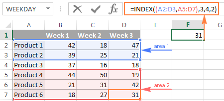
For example, the formula =INDEX((A2:D3, A5:D7), 3, 4, 2) returns the value of cell D7, which is at the intersection of the 3rd row and 4th column in the second area (A5:D7).
INDEX reference form - things to remember
- If the row_num or column_num argument is set to zero (0), an INDEX formula returns the reference for the entire column or row, respectively.
- If both row_num and column_num are omitted, the INDEX function returns the area specified in the area_num argument.
- All of the _num arguments (row_num, column_num and area_num) must refer to a cell within reference; otherwise, the INDEX formula will return the #REF! error.
Both of the INDEX formulas we've discussed so far are very simple and only illustrate the concept. Your real formulas are likely to be far more complex than that, so let's explore a few most efficient uses of INDEX in Excel.
How to use INDEX function in Excel - formula examples
Perhaps there aren't many practical uses of Excel INDEX by itself, but in combination with other functions such as MATCH or COUNTA, it can make very powerful formulas.
Source data
All of our INDEX formulas (except for the last one), we will use the below data. For convenience purposes, it is organized in a table named SourceData.
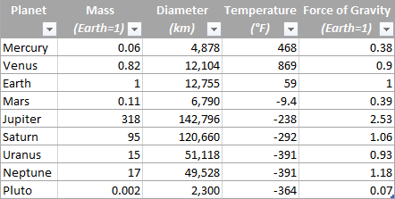
The use of tables or named ranges can make formulas a bit longer, but it also makes them significantly more flexible and better readable. To adjust any INDEX formula for your worksheets, you need only to modify a single name, and this fully makes up for a longer formula length.
Of course, nothing prevents you from using usual ranges if you want to. In this case, you simply replace the table name SourceData with the appropriate range reference.
1. Getting the Nth item from the list
This is the basic use of the INDEX function and a simplest formula to make. To fetch a certain item from the list, you just write =INDEX(range, n) where range is a range of cells or a named range, and n is the position of the item you want to get.
When working with Excel tables, you can select the column using the mouse and Excel will pull the column's name along with the table's name in the formula:
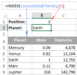
To get a value of the cell at the intersection of a given row and column, you use the same approach with the only difference that you specify both - the row number and the column number. In fact, you already saw such a formula in action when we discussed INDEX array form.
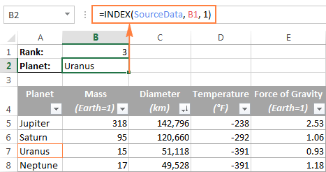
And here's one more example. In our sample table, to find the 2nd biggest planet in the Solar system, you sort the table by the Diameter column, and use the following INDEX formula:
=INDEX(SourceData, 2, 3)
Arrayis the table name, or a range reference, SourceData in this example.Row_numis 2 because you are looking for the second item in the list, which is in the 2ndColumn_numis 3 because Diameter is the 3rd column in the table.
If you want to return the planet's name rather than diameter, change column_num to 1. And naturally, you can use a cell reference in the row_num and/or column_num arguments to make your formula more versatile, as demonstrated in the screenshot below:
2. Getting all values in a row or column
Apart from retrieving a single cell, the INDEX function is able to return an array of values from the entire row or column. To get all values from a certain column, you have to omit the row_num argument or set it to 0. Likewise, to get the entire row, you pass empty value or 0 in column_num.
Such INDEX formulas can hardly be used on their own, because Excel is unable to fit the array of values returned by the formula in a single cell, and you would get the #VALUE! error instead. However, if you use INDEX in conjunction with other functions, such as SUM or AVERAGE, you will get awesome results.
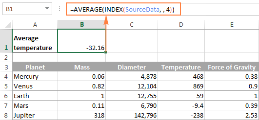
For example, you could use the following formula to calculate the average planet temperature in the Solar system:
=AVERAGE(INDEX(SourceData, , 4))
In the above formula, the column_num argument is 4 because Temperature in the 4th column in our table. The row_num parameter is omitted.
In a similar manner, you can find the minimum and maximum temperatures:
=MAX(INDEX(SourceData, , 4))
=MIN(INDEX(SourceData, , 4))
And calculate the total planet mass (Mass is the 2nd column in the table):
=SUM(INDEX(SourceData, , 2))
From practical viewpoint, the INDEX function in the above formula is superfluous. You can simply write =AVERAGE(range) or =SUM(range) and get the same results.
When working with real data, this feature may prove helpful as part of more complex formulas you use for data analysis.
3. Using INDEX with other functions (SUM, AVERAGE, MAX, MIN)
From the previous examples, you might be under an impression that an INDEX formula returns values, but the reality is that it returns a reference to the cell containing the value. And this example demonstrates the true nature of the Excel INDEX function.
Since the result of an INDEX formula is a reference, we can use it within other functions to make a dynamic range. Sounds confusing? The following formula will make everything clear.
Suppose you have a formula =AVERAGE(A1:A10) that returns an average of the values in cells A1:A10. Instead of writing the range directly in the formula, you can replace either A1 or A10, or both, with INDEX functions, like this:
=AVERAGE(A1 : INDEX(A1:A20,10))
Both of the above formulas will deliver the same result because the INDEX function also returns a reference to cell A10 (row_num is set to 10, col_num omitted). The difference is that the range is the AVERAGE / INDEX formula is dynamic, and once you change the row_num argument in INDEX, the range processed by the AVERAGE function will change and the formula will return a different result.
Apparently, the INDEX formula's route appears overly complicated, but it does have practical applications, as demonstrated in the following examples.
Example 1. Calculate average of the top N items in the list
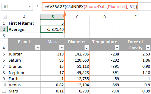
Let's say you want to know the average diameter of the N biggest planets in our system. So, you sort the table by Diameter column from largest to smallest, and use the following Average / Index formula:
=AVERAGE(C5 : INDEX(SourceData[Diameter], B1))
Example 2. Sum items between the specified two items
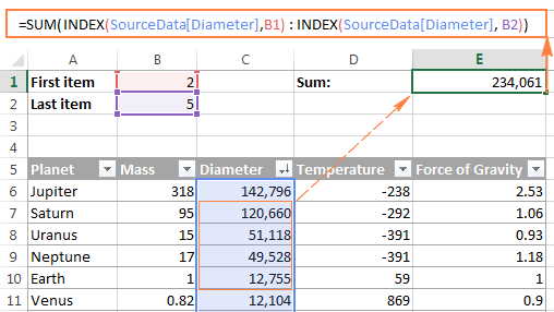
In case you want to define the upper-bound and lower-bound items in your formula, you just need to employ two INDEX functions to return the first and the last item you want.
For example, the following formula returns the sum of values in the Diameter column between the two items specified in cells B1 and B2:
=SUM(INDEX(SourceData[Diameter],B1) : INDEX(SourceData[Diameter], B2))
4. INDEX formula to create dynamic ranges and drop-down lists
As it often happens, when you start organizing data in a worksheet, you may not know how many entries you will eventually have. It's not the case with our planets table, which seems to be complete, but who knows...
Anyway, if you have a changing number of items in a given column, say from A1 to An, you may want to create a dynamic named range that includes all cells with data. At that, you want the range to adjust automatically as you add new items or delete some of the existing ones. For example, if you currently have 10 items, your named range is A1:A10. If you add a new entry, the named range automatically expands to A1:A11, and if you change your mind and delete that newly added data, the range automatically reverts to A1:A10.
The main advantage of this approach is that you do not have to constantly update all formulas in your workbook to ensure they refer to correct ranges.
One way to define a dynamic range is using Excel OFFSET function:
=OFFSET(Sheet_Name!$A$1, 0, 0, COUNTA(Sheet_Name!$A:$A), 1)
Another possible solution is to use Excel INDEX together with COUNTA:
=Sheet_Name!$A$1:INDEX(Sheet_Name!$A:$A, COUNTA(Sheet_Name!$A:$A))
In both formulas, A1 is the cell containing the first item of the list and the dynamic range produced by both formulas will be identical.
The difference is in the approaches. While the OFFSET function moves from the starting point by a certain number of rows and/or columns, INDEX finds a cell at the intersection of a particular row and column. The COUNTA function, used in both formulas, gets the number of non-empty cells in the column of interest.
In this example, there are 9 non-blank cells in column A, so COUNTA returns 9. Consequently, INDEX returns $A$9, which is the last used cell in column A (usually INDEX returns a value, but in this formula, the reference operator (:) forces it to return a reference). And because $A$1 is our starting point, the final result of the formula is the range $A$1:$A$9.
The following screenshot demonstrates how you can use such Index formula to create a dynamic drop-down list.
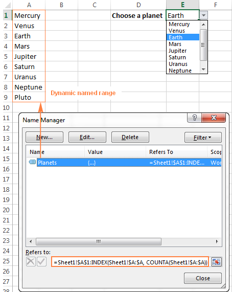
Tip. The easiest way to create an expandable dynamic data validation list is dropdown from a table. In this case, you won't need any complex formulas since Excel tables are dynamic ranges per se.
You can also use the INDEX function to create dependent drop-down lists and the following tutorial explains the steps: Making a cascading drop-down list in Excel.
5. Powerful Vlookups with INDEX / MATCH
Performing vertical lookups - this is where the INDEX function truly shines. If you have ever tried using Excel VLOOKUP function, you are well aware of its numerous limitations, such as inability to pull values from columns to the left of the lookup column or 255 chars limit for a lookup value.
The INDEX / MATCH liaison is superior to VLOOKUP in many respects:
- No problems with left vlookups.
- No limit to the lookup value size.
- No sorting is required (VLOOKUP with approximate match does require sorting the lookup column in ascending order).
- You are free to insert and remove columns in a table without updating every associated formula.
- And the last but not the least, INDEX / MATCH does not slow down your Excel like multiple Vlookups do.
You use INDEX / MATCH in the following way:
For example, if we flip our source table so that Planet Name becomes the right-most column, the INDEX / MATCH formula still fetches a matching value from the left-hand column without a hitch.
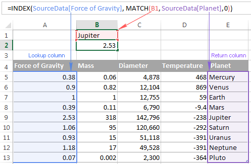
For more tips and formula example, please see the Excel INDEX / MATCH tutorial.
6. Excel INDEX formula to get 1 range from a list of ranges
Another smart and powerful use of the INDEX function in Excel is the ability to get one range from a list of ranges.
Suppose, you have several lists with a different number of items in each. Believe me or not, you can calculate the average or sum the values in any selected range with a single formula.
First off, you create a named range for each list; let it be PlanetsD and MoonsD in this example:
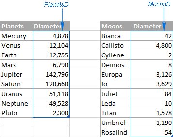
I hope the above image explains the reasoning behind the ranges' names : ) BTW, the Moons table is far from complete, there are 176 known natural moons in our Solar System, Jupiter alone has 63 currently, and counting. For this example, I picked random 11, well... maybe not quite random - moons with the most beautiful names : )
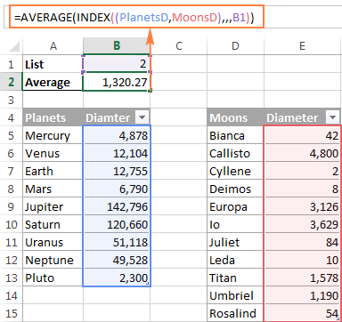
Please excuse the digression, back to our INDEX formula. Assuming that PlanetsD is your range 1 and MoonsD is range 2, and cell B1 is where you put the range number, you can use the following Index formula to calculate the average of values in the selected named range:
=AVERAGE(INDEX((PlanetsD, MoonsD), , , B1))
Please pay attention that now we are using the Reference form of the INDEX function, and the number in the last argument (area_num) tells the formula which range to pick.
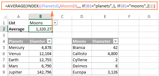
In the screenshot below, area_num (cell B1) is set to 2, so the formula calculates the average diameter of Moons because the range MoonsD comes 2nd in the reference argument.
If you work with multiple lists and don't want to bother remembering the associated numbers, you can employ a nested IF function to do this for you:
=AVERAGE(INDEX((PlanetsD, MoonsD), , , IF(B1="planets", 1, IF(B1="moons", 2))))
In the IF function, you use some simple and easy-to-remember list names that you want your users to type in cell B1 instead of numbers. Please keep this in mind, for the formula to work correctly, the text in B1 should be exactly the same (case-insensitive) as in the IF's parameters, otherwise your Index formula will throw the #VALUE error.
To make the formula even more user-friendly, you can use Data Validation to create a drop-down list with predefined names to prevent spelling errors and misprints:
Finally, to make your INDEX formula absolutely perfect, you can enclose it in the IFERROR function that will prompt the user to choose an item from the drop-down list if no selection has been made yet:
=IFERROR(AVERAGE(INDEX((PlanetsD, MoonsD), , , IF(B1="planet", 1, IF(B1="moon", 2)))), "Please select the list!")
This is how you use INDEX formulas in Excel. I am hopeful these examples showed you a way to harness the potential of the INDEX function in your worksheets. Thank you for reading!
 by
by
118 comments
Hi,
I have seen videos to populate pivot based on the value selection in the drop down using Index and Match function. My data is tricky not able to replicate the same issue. Below are the columns of info I have in the spread sheet:
Dept Month Target Actual Difference
Mktg Jan-18 100 80 20
Mktg Feb-18 120 118 2
Mktg Mar-18 90 94 4
TeleM Jan-18 200 210 10
TeleM Feb-18 150 148 2
TeleM Mar-18 110 103 7
I want my chart to change dynamically. Could you please help how to write the Index Formula. I want to display the chart data by for selected period by dept. I will select the dept and then the range of the periods which will display the chart. Since I have multiple times dept and month are coming in the data spreadsheet it is not giving the right result.
Hi,
can we use INDEX to select the default value of a list in data validation?
for example in below list
A1 Select one
A2 AA
A3 BB
A4 CC
by default, the drop list in D1 which is created by data validation >list
shows select one/
Index match on multiple criteria with multiple sheets
i have a workbook with 4 sheets 1st three are Jan, Feb, Mar and 4th one is home. Columns are style no., qty and unit price. i want to check index match the unit price of mentioned style number from all three sheets. Like i want a formula in HOME sheet in cell C2 which see style no. in cell A2 and then check it's unit price in all three sheets and put unit price of matched style no.
Three sheets Jan, Feb, Mar are like this.
Style No. Qty Unit Price
WTC123456 456 45,000
WTB281654 1000 65,000
HOME Sheet.
Style No. Qty Unit Price
WTC123456 456 here i want formula
WTB281654 1000
because some styles are put in Jan and some are in Feb so on. but home sheet has all the styles no.
so actually i have 12 sheets of 12 months
Thanks
Hi,
I want to write a VBA function making use of LINEST excel function to calculate some tstats for the slope. I know that i have to combine the INDEX function with the LINEST function, but i don't know how. Can anyone help?
Hi,
I want to write a VBA function making use of LINEST excel function to calculate some tstats for the slope. I know that i have to combine the INDEX function with the LINEST function, but i don't know how. Can anyone help?
how can i use index formula. in multiple table in one sheet
Am struggling to understand how to construct a formula that populates the "grades" column below by reading the "rounded" column content and returning the value in the "Grade" column if the value in the "rounded" column is equal to or greater than the value in the "From" and is equal to or less than the value in the "To" columns.
Any help appreciated:
rounded grades
165,000 ?
120,000 ?
110,000 ?
100,000 ?
100,000 ?
90,000 ?
90,000 ?
88,580 ?
85,000 ?
80,000 ?
From To Grade
160,000 170,000 A1
150,000 159,999 A2
140,000 149,999 A3
130,000 139,999 A4
120,000 129,999 A5
110,000 119,999 A6
100,000 109,999 A7
90,000 99,999 A8
85,000 89,999 B1
80,000 84,999 B2
75,000 79,999 B3
70,000 74,999 B4
65,000 69,999 B5
I am building a task list that needs to populate a "dashboard". There is a row in each task labeled "launch" that has a date associated with in the neighboring column. Then in the same column as "launch" there are a list of activities that has a list of corresponding "date completed". The dashboard has columns that match the activity title and the rows have the matching campaign. I'm currently using this function: =IF(ISERROR(INDEX(ALLCAMPS,SMALL(IF(ACTIVITY=$R$1,ROW(Complete_Date)),ROW(1:1)),12)),"",INDEX(ALLCAMPS,SMALL(IF(ACTIVITY=$R$1,ROW(Complete_Date)),ROW(1:1)),12)) with delete + shift + enter. It logs down my system. Is there a better way to do?
Hello,
If I’ve understood your task correctly, please try to use the modified formula below:
=IFERROR(INDEX(ALLCAMPS,SMALL(IF(ACTIVITY=$R$1,ROW(Complete_Date)),ROW(1:1)),12),"")
If this doesn’t work either, I’m afraid you’ll need to use a special macro then. We can’t help you with this since we do not cover the programming area (VBA-related questions). In this case please try to find the solution in VBA sections on mrexcel.com or excelforum.com.
I do hope you’ll manage to solve this task!
I have a schedule for 10 teams playing on 5 boards. They play 3o days and play 2 games each day, against different teams.
Left column are the dates, then to the right is what teams play each other and the board they play on above the teams.
I would post the schedule but do not see where I can post it.
I presently have a chart that I populate manually and want to do automatically depending upon what the date is, whether the 1st or 2nd game is being played.
I tried index, match, vlookup and cannot get any of them to work with the schedule I have.
What do you suggest I do? Hopefully I explained what I'm trying to do.
Thanks,
Jim
Estimated. Sq. Ft Estimated Capex Spend (£)
2,000 185,000
3,500 436,000
5,000 660,000
how do i find whats estimated capex spend for example 2500 sq ft based on the data above. what formula could i use to get an estimate?
Hi There
I have an employee data base, i have to send every week the manpower list each dept.
i want to create the drop down list by dept. when i select any dept my worksheet should the employees names in that dept.
thanks your help
Hello,
I have two columns (A and B) and that they are reference columns. I need to get the columns (C and D) are sorted according to the ref. column B using INDEX and/or MATCH functions. For instance:
No. B C D
= = = =
1 A 2 4
2 C 1 2
3 E 3 1
4 C 4 3
After sorting according to column B the columns C and D it becomes below:
No. B C D
== = = =
1 A C E
2 C A C
3 E E C
4 B C A
How to do this using functions (not normal or custom sorting) in Excel?
Thank you so much in advance.
Hello,
I have a list with 2 columns:
A:text
B:number
I wanted to
1- select records that have value 'USD'in column A (This outputs a range include recores that value of column A is 'USD')
2- Sum the column B values on range which specified in previuse step.
HOW TO DO THIS IN EXCEL USING FUNCTIONS?
thanks before
Good day
i have a challenge . been working on a report card, but i can't go through :(
NAME ENG MATHS ADMA BIO GEO CIV PHY CHE AVG PSN
BRIAN 55 3 66 2 63 2 72 2 55 3 71 2 83 1 80 1 427 68 8
BKALUMO 65 2 52 3 0 FAIL 65 2 70 2 60 2 88 1 50 3 400 56 16
IAN 70 2 24 FAIL 36 FAIL 50 3 58 3 71 2 75 1 18 FAIL 360 50 22
TREVIS 88 1 54 3 51 3 80 1 70 2 77 1 90 1 72 2 477 73 3
GRIFFINS 68 2 26 FAIL 51 3 46 4 59 3 77 1 70 2 60 2 385 57 1 HARRISON58 3 12 FAIL 34 FAIL 54 3 55 3 71 2 75 1 40 4 353 50 25
ROSTEN 78 1 42 4 45 4 58 3 74 2 63 2 85 1 80 1 438 66 7
VICTOR 78 1 56 3 60 2 56 3 59 3 83 1 85 1 24 FAIL 421 63 9
GABRIEL 48 4 38 FAIL 33 FAIL 52 3 40 4 49 4 75 1 12 FAIL 302 43 28
The card works like this . a teacher will enter the mark for a pupil then it will calculate the grade ie 1-9(fail). and also calculates the best 6 subjects including english as shown in the 3rd last column.(SUM(LARGE(E3:Q3,{1,2,3,4,5}))+C3)
i want to now add a column that will calculate the points (sum of best grade). i have tried alot of formulars but the challenges comes because the grades where found by a formular and are not in a range (in different columns)
=SUM(SMALL(range,{1,2,3,4,5}))+M34 - this formular isnt giving an answer but an error ### #num!. am stuck on how to go about it. i noticed it could be because the grades for a particular pupil are in different columns and are a result of a formular.
Please help. Thanks in advance
I am trying to retrieve the values from a range that match two criteria (A2, C2). I get only the first one, but I want them all in a dropdown list.
=INDEX(tbEmployee[Employee],MATCH($A$2&$C$2,INDEX(tbEmployee[Country]&tbEmployee[Category],,),0),0)
What shall I do?
Hi, Anastasia,
Try VLOOKUP function, it can return values based on few criteria.
If I would like to sum the values of different individual columns based on row criteria then which formula should I use?
Example:
Name A1 Loc A2 Loc A1 Loc A2 Loc
ABC 5 7 8 5
XYZ 6 8 9 6
PQR 3 9 6 3
I want sum of XYZ values of A1 location
Perhaps you can help me out. I am using the following array formula {=INDEX(ASSETP,SMALL(IF(STATP=$A$10,ROW(ASSETP)MIN(ROW(ASSETP))+1),ROWS($B10:B$10)))}
to display vertically instances of asset #'s if they equal the status in cell A10. The formula works great. The cells in the "STATP" range are formulas to determine the status. =IF(K5="","L","X"). Later I realized that I needed to improve the status formula by checking for cost of the asset. I changed the status formulas to determine if cost was $500.
=IF(AND(K6="",H6>499.99),"L",IF(AND(K6="",H6<500),"L2","X"))
The status formula works fine, but my array formulas no longer work the way I expected. If I put the Status formulas back to original the array formulas work as expected.
SOLVED. When I changed the status formula one of the cells in the STATP range, gave an error as its result. This caused the array formulas to not work as expected. Once I corrected the error all array formulas worked as expected.
Hi,
=INDEX($E2:$E$300,MATCH("PE",$D2:$D$300,0))
=INDEX($E2:$E$300,MATCH("CE",$D2:$D$300,0))
I am using above 2 formulas to extract data from E2:E300 for matching two words like CE and PE, which is situated in column D2:D300. I want result for PE in column F2 and drag down. Another CE result want in column G2 and down. But the CE word starts from row above 100 in column E and when I drag it in column G2 and down I am getting incorrect match. But getting correct result for PE.
I need some help with the formula (combination of Index and Match)- If I have row ass Quarters (B2:G2) and business listed in Column B- How can add total for business by Quarter by just changing the Quarter name in AI cell.
Hi Really struggling to source the correct formula required.
I have a table that has data entered including customer reference numbers and dates. the reference number can be entered several times in no particular order.
I want to lookup the reference number in one column, check that a date has been entered against all entries in another column and then return a Yes, No response.
Any help appreciated
Hi,
I would like to create a inventory file with condition as follow.
1) multiple products/items in one worksheet as follow
2) inventory use first in first out method to calculate col F,G,H.
Is there any formula in column F, G & H that can automatic calculate.
B C D E F G H
1 Description/Cost/QtyIn/QtyOut/QtyBal/BalAmt/QtyOutAmt
2 Product A 10 416 416 $4,160 $0
3 Product B 20 400 400 $8,000 $0
4 Product A 200 216 $2,160 200*10=$2,000 [E4*C2]
5 Product B 250 150 $3,000 250*20=$5,000 [E5*C3]
6 Product A 12 150 366 $3,960 $0
7 Product B 50 100 $2,000 50*20=$1,000 [E7*C3]
8 Product A 300 66 $792 (216*10)+(84*12)=$3,168
9 Product C 15 200 200 $3,000 $0
10 Product B 22 200 300 $6,400 $0
11 Product A 50 16 $192 $600
12 Product C 15 100 300 $4,500 $0
13 Product B 150 150 $3,300 $3,100
14 Product C 150 150 $2,250 $2,250
15 Product A 10 300 316 $3,192 $0
In Example 2 (Sum items between the specified two items)
you used the following formula
=SUM(INDEX(SourceData[Diameter],B1) : INDEX(SourceData[Diameter], B2))
is there a way i can add another condition? I want to only sum every second number in the range specified in the abovementioned formula?
so in your example 2, the answer will be 120,670+0+49,528+0 = 170,188
Thanks
Nicholas
I have to say your explanation and examples of the index function is the best I have seen.
Very clear and easy to follow.
Thank you so much!
Bruce
used a simpler approach, two SUMIFs
=sumif(B4:CH4,"="&Today(),B5:CH5)+sumif(B4:CH4,">"&Today(),B5:CH5)
gave me the answer I needed
I have a table with row 1 being dates from July thru to end of October and row 2 indicates whether a person is working (1) or not (0). I am trying to get my index/match formula to auto update to show how many days between today and the end of October the person is working. I have the following, but end up with #REF :-(
=sum(index(B4:CH4,2,match(today(),b4:ch4,0)):index(b4:ch4,2,85)
Thanks for any help
Date Name Brand Date Name Brand
are the entries.
A B C D E F G H
1/1/16 ALEX SONY 2/1/16 JOHN DELL ? ?
A to C and D to E are consecutive data categories.
I want to return in Cell G1 the name of the Person who made the sale at the latest date (JOHN).
And return in Cell H1 the name of the Brand for which the sale was done (DELL).
Kindly help.
Hellow all,
I have two questions,please have a look and let me know is there anyway to find the solution,
1. I have two tables each having 37X12 rows and columns, First row and first column is having names for the corresponding data.Here the question is, i need to sort out column 1 data (which is having same names for two tables) from the reaming 35 columns of the two tables based on max, avg and min values. it is the combination of index, match for max min and avg, but no idea how to give the reference for two tables at a time to see max min and avg values for column data.
2. I have 15 matrices, each of the matrix is having 1833x1833 rows and columns. Here the data need to be sort out for specific rows and columns say for eg. between 500 to 1000. i need to sum these columns and rows by looking the sheet name and no idea how to specify the range to lookup and sum the data.
Looking for the solution,
Thanks, Subbareddy.
I am trying to use the index function to display a dollar amount listed in a table in the month that it will be billed for. I have multiple projects and when the formula is dragged down to the next project, the index gets off because the projects have different start dates. Is there a better way to have the index start at the first billing month other than copying the formula from the previous project to the first billing month of the next project?
Thanks.
Hi,
How to set ascending order date format with using formula to another column.
Example: all dated A1:A20
Ascending another column like B1:B20
Thanks & Regards,
Sri
I'm trying to reference a cell in another workbook without success. I think my best way forward is to use Indirect() but have also tried Index() without success.
It seems to be failing on the external file location as such:
The entire cell reference is as such"
"http://apollo.omega.dce-eir.net/contentserverdav/nodes/3161757/[BIASDetailedVRFtracker.xlsm]alignment!$D$12"
My Indirect call is as follows:
Indirect("'http://apollo.omega.dce-eir.net/contentserverdav/nodes/3161757/[BIASDetailedVRFtracker.xlsm]alignment'!$D$12")
It is failing on:
http://apollo.omega.dce-eir.net/contentserverdav/nodes/3161757/
Hello,
I am trying to sum multiple columns that have months has my headers. When we close on another month data is updated in that column. I want to automatically sum the data in the rows without continually every month updating my sum formula at the end. Can someone please show me how to do this with Index and Match Function? I want it to be dynamic!
Thanks,
hello
The results show me the same which type it
the results:- =INDEX((A2:D3, A5:D7), 3, 4, 2)
Hello Yaseen,
This usually happens if a formula cell has a leading space or apostrophe before the equal sign; or if the Show Formulas mode is activated in the worksheet (Formulas tab > Formula Auditing). If neither is the case, please check out Excel formulas not calculating for other possible reasons and solutions.
Forgot to mention the function - use IFERROR - wrap you INDEX...MATCH functions in IFERROR - and the last part of the function will be your default value (0 or "Not found - try again"). I don't like the #REF or #N/A answers either.
For those values that are not found - wrap your INDEX...MATCH functions in this - and the last entry can be your default value (if not found). I don't like the $REF or #N/A answers either
Good morning I am trying to write an INDEX MATCH Formula that will dynamically set the INDEX lookup column based on the header column.
what I have are 2 tabs which house my base data; we will call them Table1 and Table2. then I have a third tab which populates all its data based on INDEX MATCH Formulas, we can call this tab Lookup1.
I have made the table headers in Table1 and Table2 names ranges and in my Lookup1 tab, I want the table headers to be dropdowns from one of my dataset tables. I'd like to write the INDEX MATCH formula to change it's INDEX column if I changed the header title in my table.
is this possible without VBA? I have pasted the original formula below, the part colored in red is what I want to rewrite to reference the header of it's own column, match the column of the same name in the Table1 tab and insert that as the Index lookup. I believe I might need to nest in another INDEX and/or MATCH formula to do what I want, but I am not sure.
=IF([@[Employee ID]]"",INDEX(Table1[First Name],MATCH([@[Employee ID]],Table1[Employee ID]),0),"")
I am maintaining a speadsheet which which monitors materials delivery (detailed and summary).
I have 2 worksheets (sheet1 is for detailed report & sheet2 is for summary report) in a workbook. What I want is a formula to automatically write "Delivered" in the Summary Report if all items (2 items each PO number in the example shown) are "Delivered" in the Detailed Report; and write "Partial" if one is "Delivered" and the remaining is "Undelivered".
Both tables are Named Tables, so the number of items will increase in time.
I tried to search in the forums but failed to get what I'm looking for. Would appreciate any help.
Sheet1-Detail
PONo. Project ProjCode Vendor Material Status
1 Project 1 Prj001 ABC Material 1 Delivered
1 Project 1 Prj001 ABC Material 2 Undelivered
2 Project 1 Prj001 XYZ Material 3 Delivered
2 Project 1 Prj001 XYZ Material 4 Delivered
Sheet2-Summary
PONo. Project ProjCode Vendor Status
1 Project 1 Prj001 ABC Partial
2 Project 1 Prj001 XYZ Delivered
Hi...can anyone help me use INDEX function to return a value and then drag it down to return values from other sheets in the same column ?
data1 data2 data3 data4 default average new data
44.44 26.75 83.80 68.36 33.00 65.53 65.53
i have to use sumif to add 3 of the data rows, omitting the highest and the lowest values.
Thanks
I have this file:
data1 data2 data3 data4 default average new data
44.44 26.75 83.80 68.36 33.00 65.53 65.53
I need to use sumif to sum 3 of the five data rows omitting the the highest and the lowest values
I use offset =OFFSET($G$2,MATCH(M3,$G$3:$G$15,0),1) and I get #N/A for the id that didn't match is there a way to output 0(zero) or Null instead of #n/a?
Hi Everyone. I am trying to get the min number from these set of value from Cell, D13 to D19.
With the method i use, it is going to be very tedious as i need to repeat it till D19.
Is there a way to rewrite this formula into an array where the formula will gather the number from D13-D19 and output the minimum?
=MIN(INDEX($D$2:$LK$3,MATCH($M$5,$B$2:$B$186,0),MATCH(D13,$D$1:$LK$1,0)),INDEX($D$2:$LK$3,MATCH($M$5,$B$2:$B$186,0),MATCH(D14,$D$1:$LK$1,0)))
Thank you!
What if I have a long time-series organized in by year (column 1) and month (column 2) and the value (column 3) and I want to compute seasonal averages (i.e. DJF, MAM, JJA, SON) over the entire time-series. How can I use the EXCEL average function to know to skip every 12th entry in generating the seasonal averages?
Hi, I have an Index Match formula: =INDEX(AI1233:AU1234,MATCH(AH1196,AI1233:AU1233,0), MATCH(AI1223,AI1233:AI1234,0)) the AH1196 is a drop down list of Jan 2016-Dec 2016. The budget data it pulls looks like this:
Date Jan-16 Feb-16 Mar-16
Postage xxxx xxxx xxxx
When I have Jan-16 in the drop down field, it works great. When I change the drop down to any other month, I get #REF!. Not sure how to enable the use of the drop down in the formula.
Any help will be greatly appreciated.
I have a large number of data in which I am trying to calculate weeks of supply. I am looking for a formula that will go to a specified cell (that contains my build for a specific category) then multiply last weeks sales by that build. If that does not equal 0, then I would like it to do the same thing and move on to the next cell and perform the same formula. Then continue until my result is zero, and finally count all the cells it performed this formula, giving me my weeks of supply.
Hello, Brian,
Your task needs a special solution. Sorry, we cannot help you with this.
Hi,
I failed to calculate via Index function the "Min" of dates array;
=INDEX(MIN('Dates'!N15:N35),MATCH(A4,'Students'!B15:B35,0))
Result is #N/A, though values are available in the date type and both respective cells.
Can you please help? Thanks.
Regards,
Tariq
Hello Tariq,
MIN function returns one value, so the second parameter of the INDEX function should by equal 1.
I am working with a similar formula with CTRL+SHIFT+ENTER and it works on the first cell, but when I copy down I get #NUM! errors?
{=INDEX($B$2:$B$8, SMALL(IF($A$11=$A$2:$A$8, ROW($A$2:$A$8)-ROW($A$2)+1), ROW(1:1)))}
Any ideas? Would be greatly appreciated!
Hello, Erik,
For us to be able to assist you better, please send us a small sample table with your data in Excel and the result you expect to support@ablebits.com.
Hi, whatever row your formula is in, use this at the end of your formula ROWS($C$1:C1)... If your formula is being built inside of c1
Check your cell address.Change the range.Your format is ok but change the range brother.Thanks in advance.
Hi there, I would like to find out how can i add a drop down list which will enable me to alternate functions such as Sum, Average etc when i have 10 values to add together or average?
NKOSI,
Use the IF function to switch between functions:
=IF(A1="SUM",SUM(B1:B10),AVERAGE(B1:B10))
https://support.ablebits.com/blog_samples/excel-index-function_2_switch_between_functions.xlsx
Hi there, I would like to find out how can i alternate functions such as Sum, Average etc when i have 10 rows with prices or values
Hello NKOSI,
You can use the IF function to switch between functions:
=IF(A1="SUM",SUM(B1:B10),AVERAGE(B1:B10))
https://support.ablebits.com/blog_samples/excel-index-function_2_switch_between_functions.xlsx
trying to use an existing spreadsheet's details to populate a different workbook dynamically, so that as the source workbook is updated (new lines inserted between existing data lines) these details transfer to the second workbook. The formula suggested is =INDEX('[MASTER Cluster Data Set.xlsx]Portfolio Clusters'!C4,1). The second workbook recognises that there is a new line to deal with but does not automatically display the row or details. Any suggestions what I am doing wrong? e-mail response would be appreciated.
Hello Sid,
Try use a named range with a few rows.
As sample: =INDEX(FirstBook.xlsx!ANYRANGE,6)