This tutorial explains the most common mistakes when making formulas in Excel, and how to fix a formula that is not calculating or not updating automatically.
Can someone imagine using Microsoft Excel without formulas? I believe no one can. And hardly anything could compare to the frustration caused by Excel formulas stop working all of a sudden. When this happens, a bunch of questions immediately flash across your mind. Why is my Excel formula not calculating? Why doesn't this formula update its value automatically? Is my Excel corrupt or is this due to some malicious virus? And how do I get my Excel to calculate and update formulas automatically again? Don't worry, most likely your Excel is all right, and you will get all the answers in a moment.
Excel formulas not working
Symptoms: Excel formula not working correctly, it returns an error or a wrong result.
This section provides a summary of the most common mistakes people make when creating formulas in Excel and solutions to fix them.
1. Match all opening and closing parentheses in a formula
As you know, the arguments of Excel functions are entered within the parentheses. In complex formulas, you may need to enter more than one set of parentheses, one within another, to indicate the order in which the calculations should take place. When creating such a formula, be sure to pair the parentheses properly so that you always have a right parenthesis for every left parenthesis in your formula.
Microsoft Excel displays the parentheses pairs in different colors as you enter them in a formula. If your formula is short of one or more parentheses, Excel displays an error message and suggests a correction to balance the pairs. Please see How to highlight and match parenthesis pairs for more information.
2. Enter all required arguments in an Excel function
All Excel functions have one or more required arguments. Some functions also have optional arguments, which are enclosed in [square brackets] in the formula's syntax.
A formula must contain all of the required arguments, otherwise Excel displays "You've entered too few arguments for this function" alert.
If you have entered more arguments than allowed by the formula's syntax, you will get "You've entered too many arguments for this function" error message.
3. Do not nest more than 64 functions in a formula
When nesting two or more Excel functions into each other, e.g. creating a nested IF formula, remember about the following limitations:
- In Excel 2016, Excel 2013, Excel 2010 and Excel 2007, you can use up to 64 nested functions.
- In Excel 2003 and lower, only up to 7 nested functions can be used.
4. Don't enclose numbers in double quotes
In Excel formulas, any value enclosed in double quotes is interpreted as a text string.
What it means is that if you enter a formula like =IF(A1>0, "1"), Excel will treat number 1 as text, and therefore you won't be able to use the returned 1's in other calculations. To fix this, just remove the double quotes around "1": =IF(A1>0, 1).
So, whenever you are writing a formula for numerical values, follow this simple rule: don't enclose numbers in double quotes unless you want them to be treated as text.
5. Enter numbers without any formatting
When using a number in an Excel formula, don't add any decimal separator or currency sign like $ or €.
Remember that in Excel formulas, a comma is typically used to separate a function's arguments, and the dollar sign makes an absolute cell reference.
For instance, instead of entering $50,000 in your formula, input simply 50000, and use the Format Cells dialog (Ctrl + 1) to format the output to your liking.
6. Make sure numbers are not formatted as text values
Numbers formatted as text values are another common reason for Excel formulas not working. At first sight, they look like normal numbers, but Microsoft Excel perceives them as text strings and leaves out of calculations.
The visual indicators of text-numbers are as follows:
- Numbers formatted as text are left-aligned by default, while normal numbers are right-aligned in cells.
- The Number Format box on the Home tab in the Number group displays the Text format.
- When several cells with text numbers are selected on the sheet, the Status Bar only shows Count, while usually it shows Average, Count and SUM for numbers.
- There may be a leading apostrophe visible in the formula bar, or green triangles appear in the top-left corner of the cells.
The below screenshot shows that even a simple Excel SUM formula may not work because of numbers formatted as text:

To fix this, select all problematic cells, click the warning sign, and then click Convert to Number:
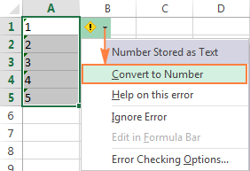
In some cases, however, neither green triangles nor the warning sign appear in cells. For example, if you enclose numeric values in double quotes in your formulas, Excel assumes you want to output a text string rather than a number.
At first sight, the following formula appears to be working fine:
=IF(A1="Good", "1", "0")
But the problem is the returned 1's and 0's are text values, not numbers! And if you reference any cells with the above formula in other formulas, those cells won't be included in calculations. As soon as you remove "" surrounding 1 and 0 in the above formula, Excel will treat the outputs as numbers and they will be calculated correctly.
If the small green triangles do not appear in cells for some other reason, look at the Number Format box on the Home tab in the Number group. If it displays Text, try clearing all formatting for the problematic cells, and set the cells' format to Number or General. If that doesn't work, you might have to create a new column, manually input the data (e.g. copy your text-numbers to Notepad, and then back to a new column), and delete the broken column.
Another possible solution is to multiply the values in the problematic column by 1 using a simple formula like =A1*1. And then, copy the formula cells and paste them as values in the same or in any other column via Paste Special > Values.
7. Separate function arguments with a proper character
Most of us are used to separating function arguments with commas. However, this does not work for everyone's Excel. The character you use to separate arguments depends on the List Separator set in your Regional Settings.
Comma is the default list separator in North America and some other countries. In European countries, comma is used as the decimal symbol and the list separator is usually set to semicolon.
For example, in North America you would write =IF(A1>0, "OK", "Not OK"), while European users of Excel should put the same formula as =IF(A1>0; "OK"; "Not OK").
So, if your Excel formulas are not working because of "We found a problem with this formula..." error, go to your Regional Settings (Control Panel > Region and Language > Additional Settings) and check what character is set as List Separator there. And then, use exactly that character to separate arguments in your Excel formulas.
8. Enclose workbook and worksheet names in single quotes
When referring to other worksheets or workbooks that have spaces or non-alphabetical characters in their names, enclose the names in 'single quotation marks'. For example,
Reference to another sheet:
=SUM('Jan Sales'!B2:B10)
Reference to another workbook:
=SUM('[2015 Sales.xlsx]Jan sales'!B2:B10)
For more information, please see How to refer to another sheet or workbook in Excel.
9. Include the full path to a closed workbook
If you are writing a formula that references a closed Excel workbook, your external reference must include the workbook name and entire path to the workbook. For example:
=SUM('D:\Reports\[Sales.xlsx]Jan'!B2:B10)
For more information, please see Creating a reference to another workbook.
If the above tips do not help, try to evaluate and debug each part of your formula individually by using the F9 key and other debugging techniques explained in the following tutorial: How to evaluate and debug formulas in Excel.
Excel formulas not updating
Symptoms: The value returned by your Excel formula does not update automatically, i.e. the formula continues to show the old value even after you've changed the values of the dependent cells.
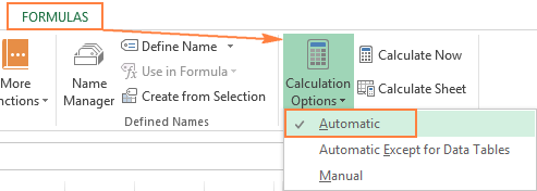
When Excel formulas are not updating automatically, most likely it's because the Calculation setting has been changed to Manual instead of Automatic. To fix this, just set the Calculation option to Automatic again.
On the Excel ribbon, go to the Formulas tab > Calculation group, click the Calculation Options button, and select Automatic:
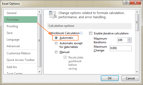
Alternatively, you can change this setting in Excel Options:
- In Excel 2003, click Tools > Options > Calculation > Calculation > Automatic.
- In Excel 2007, click Office button > Excel options > Formulas > Workbook Calculation > Automatic.
- In Excel 2010, Excel 2013, and Excel 2016, go to File > Options > Formulas > Calculation options section, and select Automatic under Workbook Calculation.
How to force Excel formulas to recalculate
If for some reason, you need to have the Calculation option set to Manual, you can force the formulas to recalculate by clicking the Calculate button on the ribbon or by using one of the following shortcuts:
To recalculate the entire workbook:
- Press F9, or
- Click the Calculate Now button on the Formulas tab > Calculation group.
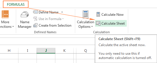
To recalculate an active sheet:
- Press Shift + F9, or
- Click Calculate Sheet on the Formulas tab > Calculation group.
To recalculate all sheets in all open workbooks, press Ctrl + Alt + F9.
If you need to recalculate only one formula on a sheet, select the formula cell, enter the editing mode either by pressing F2 or double clicking the cell, and then press the Enter key.
Excel formulas not calculating
Symptoms: A cell displays the formula, not the result.
If your Excel formula is not working because a cell displays the function instead of the calculated value, it's because one of the following reasons.
1. Show Formulas mode is turned on
The most common reason for an Excel formula not calculating is that you have inadvertently activated the Show Formulas mode in a worksheet.
To get the formula to display the calculated result, just turn off the Show Formulas mode by doing one of the following:
- Pressing the Ctrl + ` shortcut, or
- Clicking the Show Formulas button on the Formulas tab > Formula Auditing group.

2. A formula is entered as text
Another frequent reason for your Excel formula not calculating is that the formula has been formatted as text. To check this, select the formula cell, and look at the Number Format box in the Number group on the Home tab:
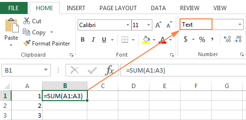
If it is the case, change the cell format to General, and while in the cell press F2 and Enter for the formula to recalculate and display the calculated value.
3. A formula cell has a leading space or apostrophe before the equal sign
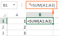
If you have inadvertently entered a space or apostrophe (') before the equal sign, Excel treats the cell contents as text, and consequently does not evaluate any formula within that cell (a leading space often appears when you copy a formula from the web). To fix this, just remove the leading space or single quote.
This is how you deal with formulas not working in Excel. If you know any other solutions to fix formulas not updating or not calculating, please do share in comments. I thank you for reading and hope to see you on our blog next week.
 by
by
438 comments
The formula for the sports spreadsheet listed above is {=sum(($A$5:$A$27=Al18)*(ISNUMBER($B$5:$B$27)),($C$5:$C$27=Al18)*(ISNUMBER($D$5:$D$27)))}
Hi Guys
I am using a formula based spreadsheet to help with team sport fixtures and have just increased my fixture listing which needs an amendment to the games played. I am trying to modify the cells its looking for to increase from A27 to A32 BUT any attempt at changing the formula translates to losing the end parenthesis {} from the formula and it then does not recognise it at all. I have tried dragging rather than correcting in the formula, what I am missing please its excel 2013
Thanks
Hi there....i've just upgraded to 365 and tried to do something in my file that i did with the 2010 version but having no success.....
We use excel for our check register.... we enter the amount in one cell., and the category number in one.....then i (used to) check enable macros
and Control C to spread the amounts to each category that are listed horizontally(columns)
i have no way of doing that now...there's probably an easier way to spread out the figures so they match the totals????
HELP!
This was so helpful. My formulas calculation were changed to manual and I don't remember how. This was lifesaving. Thanks
Hello, I am trying to calculate the total price of an item but the formula produces a slightly inaccurate result. The formula shows:
QTY ITEM COST TAX SUBTOTAL TOTAL
26 shirts $28.95 $2.90 $31.85 $827.97
The correct TOTAL should show $828.10. Can anyone help please?
I have entered the following formula:
=IF(AND(F3>TIME(6,0,0),F3<TIME(22,0,0)),"TRUE","FALSE")
F3 = [=Now()] to return the time (Cell is formatted to show time (00:00:00)
at 10:29:00 why does my formula return FALSE? when it should be TRUE...
What I require:
I want the cell with the formula in to return a figure when the time of day is between 6am and 10pm and another if it is not (Ie between 10pm and 6am)..
Anyone.....please help!!
nycccc please send formule sum and vluck
To extract due date between two given dates, I have used the following array formula
{=SMALL(IF(($G$5:$G$7=$P$1), IF(($J$5:$J$7=$P$1), ($G$5:$G$7+$J$5:$J$7), "A")), ROWS($A$5:A5))}
The due date is extracted from two distinct date column i.e. G and J
The result evaluated #NUM!
Please help to rectify the problem.
Thanks
Thanks. It helps a lot.
can anyone help me to resolve my query. I want to sum some numeric values by using excel formulae having some special charecters. for example 20+14@+36+17*+16+23? where @ means condone marks and * means fail in that particular subject
I use the =AVERAGE(IF(....)) formula.
When I click the fx button, the result is correct. Unfortunately the output into the cell is incorrect!!!!!!
Thank you for your comment, Maria,
Could you please specify the entire formula you're using in your cell?
I have a formula. It works. I copy down in the sheet. It works...up to a point. From that point on it returns the same value regardless of the inputs. The formula doesn't change:
This works:
=IF('Formal Labs'!L46="","",VLOOKUP(VLOOKUP(A46,'Formal Labs'!$A$4:$L$48,12),Parameters!$L$2:$M$15,2))
This doesn't (and any others after L47)
=IF('Formal Labs'!L47="","",VLOOKUP(VLOOKUP(A47,'Formal Labs'!$A$4:$L$48,12),Parameters!$L$2:$M$15,2))
Its on automatic calculation, I've recalculated. I've formatted all referenced cells to the same categories.
Hello -
I'm running Excel 16.20 for Mac (Office 365). My cells are all text. I have this function:
=IF(A3=A2,C2&", "&B3,B3)
The result when true is only the contents of C2. I don't get the , B3.
Any help is appreciated, thanks!
I wrote that my cells are all text, actually just the contents are text. The format of the cells is General. Thanks.
=IF(B5>'New Input'!$C$36, (((B5-'New Input'!$C$36)*'New Input'!$F$36)+(('New Input'!$C$36-'New Input'!$C$35)*'New Input'!$F$35)+(('New Input'!$C$35-'New Input'!$C$34)*'New Input'!$F$34)+(('New Input'!$C$34-'New Input'!$C$33)*'New Input'!$F$33)+(('New Input'!$C$33-'New Input'!$C$32)*'New Input'!$F$32)), IF(B5>'New Input'!$C$35, (((B5-'New Input'!$C$35)*'New Input'!$F$35)+(('New Input'!$C$35-'New Input'!$C$34)*'New Input'!$F$34)+(('New Input'!$C$34-'New Input'!$C$33)*'New Input'!$F$33)+(('New Input'!$C$33-'New Input'!$C$32)*'New Input'!$F$32)), IF(B5>'New Input'!$C$34, (((B5-'New Input'!$C$34)*'New Input'!$F$34)+(('New Input'!$C$34-'New Input'!$C$33)*'New Input'!$F$33)+(('New Input'!$C$33-'New Input'!$C$32)*'New Input'!$F$32)), IF(B5>'New Input'!$C$33, (((B5-'New Input'!$C$33)*'New Input'!$F$33)+(('New Input'!$C$33-'New Input'!$C$32)*'New Input'!$F$32)), (B5-'New Input'!$C$32)*'New Input'!$F$32))))
not working as i expect, Excel doesnt compare the values and take the decison, it keeps skipping to the FALSE value and calculates, (B5-'New Input'!$C$32)*'New Input'!$F$32) this part!
i dont even know what to do!!
please let me know if there's a problem with my formula!!
My problem here is my sum formula does not give correct answers to the subsequent row but it gives the same result while being scrolled. what is the problem?
like
2 4 5 6 17
1 3 6 2 17
what is the problem here?
You solved my "Excel formulas not updating" problem.
Thank you very much xx :)
Thanks, problem solved!
Thanks very helpful.
i love you! it helped me with my problem. :D
Thank you so much!!!
This is so helpful. Thanks a lot.
Thanks! Very helpful tips.
Activity Code Pipe Size Thickness Qty in CUM Qty in SQM.
1 0.5 25 0.0182 1.1200
1 0.5 40 0.0054 0.2228
1 0.5 50 0.0056 0.1905
1 0.5 65 0.0264 0.7130
1 0.75 25 0.0061 0.3614
1 0.75 40 0.0091 0.3620
1 0.75 50 0.0000 0.0000
1 0.75 65 0.0936 2.4614
1 0.75 75 0.0168 0.3886
1 1 25 0.0229 1.3100
1 1 40 0.0065 0.2494
1 1 50 0.0066 0.2095
1 1 65 0.0301 0.7700
1 1 100 0.0293 0.5133
1 1 125 0.0311 0.4452
1 1 150 0.1296 1.5711
1 2 50 0.5300 1.0000
1 2 65 0.4000 1.2000
1 2 75 0.0223 0.4625
1 2 100 0.0574 0.9322
1 2 125 0.2000 0.5000
1 10 150 0.3000 0.6000
1 10 300 0.4000 0.7000
1 12 50 0.5000 0.8000
1 12 100 0.2000 0.9000
1 12 200 0.3000 0.6000
1 20 75 0.4000 0.7000
1 20 150 0.5000 0.8000
1 20 300 0.3000 0.9000
and criteria are as below:
Activity Code Pipe Size Thickness
1 0.5 25
3 0.75 40
7 1 50
4 1.5 65
5 2 75
3 80
4 90
5 100
6 125
8 150
10 175
12 200
14 225
16 250
18 300
20
up to 96
How to sum of cum or sqm of specify activity, pipe size and thickness.
Hi, I have a formula that looks at cell B1 to see if it's blank, if it is, it takes the value from cell A1, but if it isn't it takes the value from cell B1....that's not the problem.
My cell B1 is blank, so should take cell A1, but the formula does not bring back the value (formula cell stays blank), unless I go to cell B1, hit F2 and enter. My calculation option is set to Automatic...
Why is this happening and what can I do to fix it?
Thanks
Thank you! I thought I was going crazy!
Hi. really hope you can help me. i want to copy a formula into a column that will multiply cell a3's formula down the column with result being sum of each row. i'm getting a3's result down the column not calculating each row appropriately.
thanks....problem solved.
Common things listed on other sites. I have functions that will not update unless you click in the formula line and hit enter (super simple COUNTIFS function based on some table data). There are no errors, they will just not calculate, period. This seems more like a problem with Excel.
What a relief! Calculation was changed to manual instead of automatic... I was ready to cry! Thank you so much!!
Hi, wondered if you can help, i have a spreadsheet. Edited the formula and its now displaying as zero even though the returned value should not be zero. Then i went and changed a figure of the precedents to get this to work and it fixed the orginial formula but now this one does not. tried updating sheets and cell formatting and no luck....any ideas? thanks
If function does not update or calculate easiest trick is to create function to new blank excel and copy it from there to existing sheet. This method copies all formatting as needed.
Thank you this helped me solve my problem. The new spreadsheet displayed the same issue, so I changed the formula.
thanks kindly, correcting to Auto Calculation, which i had mistakenly turned off, repaired my problem.
Thank you so much! I have been having this problem on and off for years. So helpful.
I have same issues as above but, my calculation options are set to automatic and my formatting is not on text - it is set to percentage. This formula works on all other years data except for 2018 data; it will not automatically populate. HELP!
Very helpful!
Thank very much
Wow, thank you - Calculation setting has been changed to Manual instead of Automatic ! Was about to scream before I read this ! 2 minutes later all sorted ! Thank you !
Thanks very helpful and it worked!
Solved after much trauma. I thought I was going mad.
I also have been running Wordperfect Quattro pro and having the same problem there and am about to investigate that.
Hooray, thank you search engines and thank you for your article in solving my problem.
When I updated the cell with new values the cell continued to show the old value. After reading this tutorial, I fixed it in 30 seconds by restoring Calculation Options back to automatic. Thank you!
None of this applies. Excel will evaluate the formula once and then stop.
Thank you!
none of the 3 above advises are working I still have the same problem that the formula is not changing to text nor numbers... can someone help please?
Great Help!
every time i change the number the font corrupted
N.B the font is Arabic
very useful
thanks a million
very helpful! & useful
thanks that is very usful
In my worksheet I continuously add a range of cells (not the entire column) using the sum formula, however if I insert a new row below my cell range but above the sum total cell, it does not recalculate the sum total. How can I update the sum total without having to adjust the cell range each and every time I insert a new row below the cell range/above the sum total cell. Thank you for your time. Victoria
Hi Victoria, try formatting the entire range as a table, that way, Excel should automatically add the new row to the table, and then update the sum. The formula for the sum would look something like this =sum(Table1[Column1])
I was having trouble with the upper formula not showing results of the formula. I updated the worksheet to a table as mentioned above and it worked!
Wow - very helpful! With 3 clicks my problem of cells not automatically updating was fixed. Thank you!!!