A while ago we started to explore the capabilities of Excel Data Validation and learned how to create a simple drop-down list in Excel based on a comma-separated list, range of cells or a named range.
Today, we are going to investigate this feature in-depth and learn how to create cascading drop down lists that display choices depending on the value selected in first dropdown. To put it differently, we will make an Excel data validation list based on the value of another list.
How to create multiple dependent dropdown in Excel
Making a multi-level dependent drop-down lists in Excel is easy. All you need is a few named ranges and the INDIRECT formula. This method works with all versions of Excel 365 - 2010 and earlier.
1. Type the entries for the drop-down lists
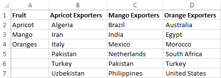
First off, type the entries you want to appear in the drop-down lists, each list in a separate column. For example, I'm creating a cascading dropdown of fruit exporters and column A of my source sheet (Fruit) includes the items of the first dropdown and 3 other columns list the items for the dependent dropdowns.
2. Create named ranges
Now you need to create names for your main list and for each of the dependent lists. You can do this either by adding a new name in the Name Manager window (Formulas tab > Name Manager > New) or typing the name directly in the Name Box.
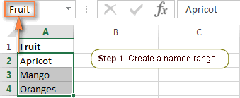
Note. Please pay attention that if your first row is sort of column header like you see in the screenshot above, you shall not include it in the named range.
For the detailed step-by-step instructions please see How to define a name in Excel.
Things to remember:
- The items to appear in the first drop-down list must be one-word entries, e.g. Apricot, Mango, Oranges. If you have items consisting of two, three or more words, please see How to create a cascading dropdown with multi-word entries.
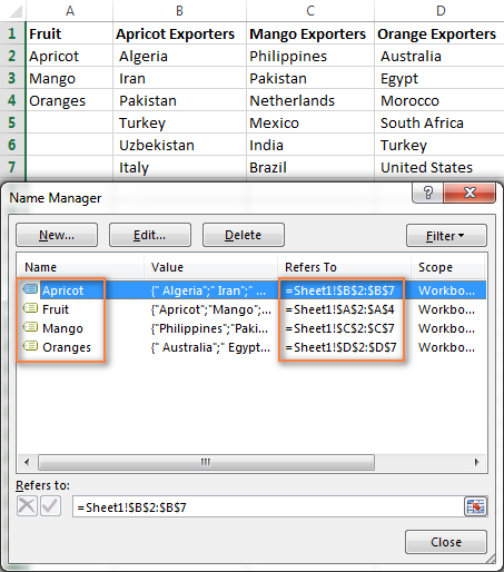
- The names of the dependent lists must be exactly the same as the matching entry in main list. For example, the dependent list to be displayed when "Mango" is selected from the first drop-down list should be named Mango.
When done, you may want to press Ctrl+F3 to open the Name Manager window and check if all of the lists have correct names and references.
3. Make the first (main) drop-down list
- In the same or in another spreadsheet, select a cell or several cells in which you want your primary drop-down list to appear.
- Go to the Data tab, click Data Validation and set up a drop-down list based on a named range in the usual way by selecting List under Allow and entering the range name in the Source box.
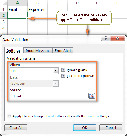
For the detailed steps, please see Making a drop down list based on a named range.
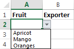
As the result, you will have a drop-down menu in your worksheet similar to this:
4. Create the dependent drop-down list
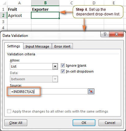
Select a cell(s) for your dependent drop-down menu and apply Excel Data Validation again as described in the previous step. But this time, instead of the range's name, you enter the following formula in the Source field:
=INDIRECT(A2)
Where A2 is the cell with your first (primary) drop-down list.
If cell A2 is currently empty, you will get the error message "The Source currently evaluates to an error. Do you want to continue?"
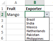
Safely click Yes, and as soon as you select an item from the first drop-down menu, you will see the entries corresponding to it in the second, dependent, drop-down list.
5. Add a third dependent drop-down list (optional)
If needed, you could add a 3rd cascading drop-down list that depends either on the selection in the 2nd drop-down menu or on the selections in the first two dropdowns.
Set up 3rd dropdown that depends on 2nd list
You can make the drop-down list of this type in the same fashion as we've just made a second dependent drop-down menu. Just remember the 2 important things discussed above, which are essential for the correct work of your cascading drop-down lists.
For instance, if you want to display a list of regions in column C depending on which country is selected in column B, you create a list of regions for each country and name it after the country's name, exactly as the country appears in second dropdown lists. For instance, a list of Indian regions should be named "India", a list of Chines regions - "China", and so on.
After that, you select a cell for the 3rd dropdown (C2 in our case) and apply Excel Data Validation with the following formula (B2 is the cell with the second drop-down menu that contains a list of countries):
=INDIRECT(B2)
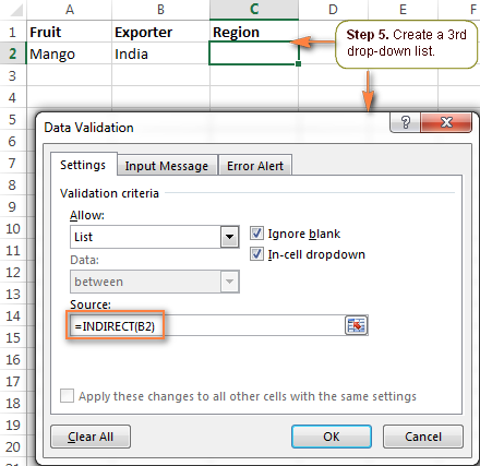
Now, each time you select India under the list of countries in column B, you will have the following choices in the third drop-down:
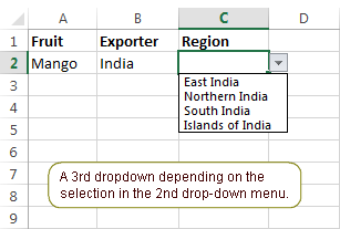
Note. The displayed list of regions is unique for each country but it does not depend on the selection in the first drop-down list.
Create a third dropdown dependent on the first two lists
If you need to create a cascading drop down menu that depends on the selections both in the first and second drop-down lists, then proceed in this way:
- Create additional sets of named ranges, and name them for the word combinations in your first two dropdowns. For example, you have Mango, Oranges, etc. in the 1st list and India, Brazil, etc. in the 2nd. Then you create named ranges MangoIndia, MangoBrazil, OrangesIndia, OrangesBrazil, etc. These names should not contain underscores or any other additional characters.
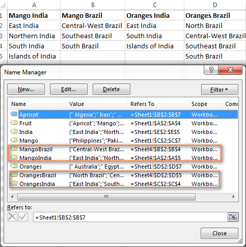
- Apply Excel Data Validation with the INDIRECT SUBSTITUTE formula that concatenates the names of the entries in the first two columns, and removes the spaces from the names. For example, in cell C2, the data validation formula would be:
=INDIRECT(SUBSTITUTE(A2&B2," ",""))Where A2 and B2 contain the first and second dropdowns, respectively.
As the result, your 3rd drop-down list will display the regions corresponding to the Fruit and Country selected in the first 2 drop-down lists.
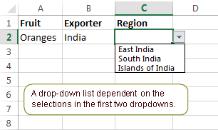
This is the easiest way to create cascading drop-down boxes in Excel. However, this method has a number of limitations.
Limitations of this approach:
- The items in your primary drop-down list must be one-word entries. See how to create cascading drop-down lists with multi-word entries.
- This method won't work if the entries in your main drop-down list contain characters not allowed in range names, such as the hyphen (-), ampersand (&), etc. The solution is to create a dynamic cascading dropdown that does not have this restriction.
- Drop-down menus created in this way are not updated automatically i.e. you will have to change the named ranges' references every time you add or remove items in the source lists. To get over this limitation, try making a dynamic cascading drop down list.
Create cascading drop-down lists with multi-word entries
The INDIRECT formulas that we used in the example above can handle one-word items only. For example, the formula =INDIRECT(A2) indirectly references cell A2 and displays the named range exactly with the same name as is in the referenced cell. However, spaces are not allowed in Excel names, which is why this formula won't work with multi-word names.
The solution is to use the INDIRECT function in combination with SUBSTITUTE like we did when creating a 3rd dropdown.
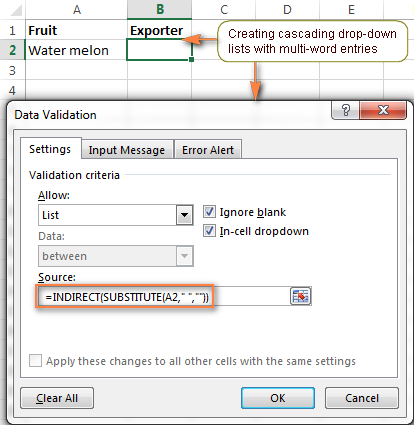
Suppose you have Water melon among the products. In this case, you name a list of water melon exporters with one word without spaces - Watermelon.
Then, for the second dropdown, apply Excel Data Validation with the following formula that removes the spaces from the name in cell A2:
=INDIRECT(SUBSTITUTE(A2," ",""))
How to prevent changes in the primary drop down list
Imagine the following scenario. Your user has made the selections in all of the drop-down lists, then they changed their mind, went back to the first list, and chose another item. As the result, the 1st and 2nd selections are mismatched. To prevent this from happening, you may want to block any changes in the first drop-down list as soon as a selection is made in the second list.
To do this, when creating the first dropdown, use a special formula that will check whether any entry is selected in the second drop down menu:
=IF(B2="", Fruit, INDIRECT("FakeList"))
Where B2 contains the second dropdown, "Fruit" is the name of the list that appears in the first drop-down menu, and "FakeList" is any fake name that does not exist.
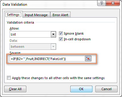
Now, if any item is selected in the 2nd drop-down list, no choices will be available when the user clicks on the arrow next to the first list.
Creating dynamic cascading drop-down lists in Excel
The main advantage of a dynamic Excel dependent drop-down list is that you are free to edit the source lists and your drop-down boxes will get updated on the fly. Of course, creating dynamic dropdowns requires a bit more time and more complex formulas, but I believe this is a worthy investment because once set up, such drop-down menus are real pleasure to work with.
As with almost anything in Excel, you can achieve the same result in several ways. In particular, you can create a dynamic dropdown using a combination of OFFSET, INDIRECT and COUNTA functions or a more resilient INDEX MATCH formula. The latter is my preferred way because it provides numerous advantages, the most essential of which are:
- You have to create 3 named ranges only, no matter how many items there are in the main and dependent lists.
- Your lists may contain multi-word items and any special chars.
- The number of entries can vary in each column.
- The entries' sort order does not matter.
- Finally, it's very easy to maintain and modify the source lists.
Okay, enough theory, let's get to practice.
1. Organize your source data in a table
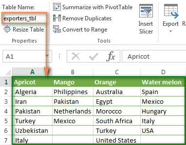
As usual, the first thing for you to do is to write down all the choices for your drop-down lists in a worksheet. This time, you will have store the source data in an Excel table. For this, once you have entered the data, select all of the entries and press Ctrl + T or click Insert tab > Table. Then type a name of your table in the Table Name box.
The most convenient and visual approach is to store the items for the first drop-down as table headers, and the items for the dependent dropdown as table data. The screenshot below illustrates the structure of my table, named exporters_tbl - the fruit names are table headers and a list of exporting countries is added under the corresponding fruit name.
2. Create Excel names
Now that your source data is ready, it's time to set up named references that will dynamically retrieve the correct list from your table.
2.1. Add a name for the table's header row (main dropdown)
To create a new name that references the table header, select it and then either click Formulas > Name Manager > New or press Ctrl + F3.
Microsoft Excel will use the built-in table reference system to create the name of the table_name[#Headers] pattern.
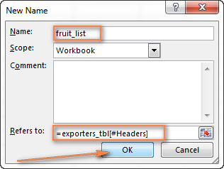
Give it some meaningful and easy to remember name, e.g. fruit_list, and click OK.
2.2. Create a name for the cell containing the first drop-down list
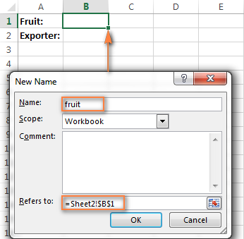
I know that you don't have any dropdown yet :) But you have to choose the cell to host your first dropdown and create a name for that cell now because you will need to include this name in the third name's reference.
For example, my first drop-down box is reside in cell B1 on Sheet 2, so I create a name for it, something simple and self-explanatory like fruit:
Tip. Use appropriate cell references to copy drop-down lists across the worksheet.
Please be sure to read the following few paragraphs carefully because this a very useful tip you that don't want to miss. Thanks a lot to Karen for posting it!
If you plan to copy your drop-down lists to other cells, then use mixed cell references when creating the name for the cell(s) with your first drop-down list.
For the drop-downs to copy correctly to other columns (i.e. to the right), use relative column (without the $ sign) and absolute row (with $) references like = Sheet2!B$1.
As the result, B1's dependent drop down list will appear in cell B2; C1's dependent drop-down will display in C2, and so on.
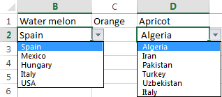
And if you plan to copy the dropdowns to other rows (i.e. down the column), then use absolute column (with $) and relative row (without $) coordinates like = Sheet2!$B1.
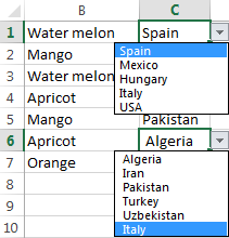
To copy a drop-down cell in any direction, use a relative reference (without the $ sign) like = Sheet2!B1.
2.3. Create a name to retrieve the dependent menu's entries
Instead of setting up unique names for each of the dependent lists like we did in the previous example, we are going to create one named formula that is not assigned to any particular cell or a range of cells. It will retrieve the correct list of entries for the second dropdown depending on which selection is made in the first drop-down list. The main benefit of using this formula is that you won't have to create new names as you add new entries to the first drop-down list - one named formula covers them all.
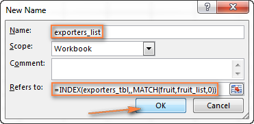
You create a new Excel name with this formula:
=INDEX(exporters_tbl,,MATCH(fruit,fruit_list,0))
Where:
exporters_tbl- the name of the table (created in step 1);fruit- the name of the cell containing the first drop-down list (created in step 2.2);fruit_list- the name referencing the table's header row (created in step 2.1).
I gave it a name exporters_list, as you see in the screenshot below.
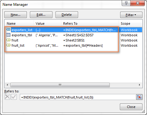
Well, you have already done the major part of the work! Before getting to the final step, it may be a good idea to open the Name Manager (Ctrl + F3) and verify the names and references:
3. Set up Excel Data Validation
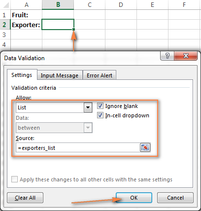
This is actually the easiest part. With the two named formulas in place, you set up Data Validation in the usual way (Data tab > Data validation).
- For the first drop-down list, in the Source box, enter =fruit_list (the name created in step 2.1).
- For the dependent drop-down list, enter =exporters_list (the name created in step 2.3).
Done! Your dynamic cascading drop-down menu is accomplished and will update automatically reflecting the changes you've made to the source table.
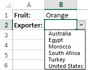
This dynamic Excel dropdown, perfect in all other respects, has one shortcoming - if the columns of your source table contain a different number of items, the blank rows will appear in your menu like this:
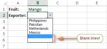
Exclude blank rows from the dynamic cascading dropdown
If you want to clean any blank lines in your drop-down boxes, you will have to take a step further and improve the INDEX / MATCH formula used to create the dependent dynamic drop-down list.
The idea is to use 2 INDEX functions, where the first gets the upper-left cell and the second returns the lower-right cell of the range, or the OFFSET function with nested INDEX and COUNTA. The detailed steps follow below:
1. Create two additional names
Not to make the formula too bulky, create a couple of helper names with the following simple formulas first:
- A name called col_num to reference the selected column number:
=MATCH(fruit,fruit_list,0) - A name called entire_col to reference the selected column (not the column's number, but the entire column):
=INDEX(exporters_tbl,,col_num)
In the above formulas, exporters_tbl is your source table's name, fruit is the name of the cell containing the first dropdown, and fruit_list is the name referencing the table's header row.
2. Create the named reference for the dependent dropdown
Next, utilize either of the below formulas to create a new name (let's call it exporters_list2) to be used with the dependent drop-down list:
=INDEX(exporters_tbl,1,col_num) : INDEX(exporters_tbl, COUNTA(entire_col), col_num)
=OFFSET(INDEX(exporters_tbl,1,col_num),0,0,COUNTA(entire_col))
3. Apply Data Validation
Finally, select the cell containing the dependent dropdown and apply Data Validation by entering = exporters_list2 (the name created in the previous step)in the Source box.
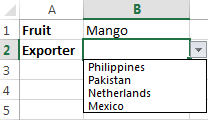
The screenshot below shows the resulting dynamic drop-down menu in Excel where all blank lines are gone!
Note. When working with dynamic cascading drop down lists created with the above formulas, nothing prevents the user from changing the value in the first dropdown after making the selection in the second menu, as a result, the choices in the primary and secondary dropdowns may mismatch. You can block changes in the first box after a selection is made in the second one by using either VBA or complex formulas suggested in this tutorial.
This is how you create an Excel data validation list based on the values of another list. Please feel free to download our sample workbooks to see the cascading drop-down lists in action. Thank you for reading!
Practice workbook for download
Cascading Dropdown Sample 1- easy version
Cascading Dropdown Sample 2 - advanced version without blanks
 by
by
319 comments
Hello,
I followed your article closely and have managed to achieve what I intended. Thanks a ton.
However, I am unable to apply it to other cells (rows below) if i drag the bottom right of the cell where the formulae are working well.
What am I doing wrong?
Thanks in advance,
Shreeram
I after something similar. My drop down list is either BPay or Bank Deposit. If they select BPay, I want Biller code and Reference to appear in 2 different cells below. Like wise, if Bank Deposit is selected, I want Acc No, Acc Name, Bank Name and BSB to appear in 4 cells below.
Is this possible?
Thank you
Dan
Hi there!
I have been looking for a way where by if i enter an item's name ie. Bag, in the next cell the price ie. $19.50 would automatically appear. Is it possible on excel?:)
Thank you!
-Sarah
Svetlana,
So I have two columns, each being a drop-down list. I want to be able to change either list, based on the choice in the other cell.
For example, if i choose "apple" from the drop down list in A1, B1 will then read "red".
But conversely, i would like to choose "pink" from the drop down list in B1, and have it change A1 to "peach".
And this applies back and forth so that each column, A and B will be updated no matter which list is chosen from, all the while keeping them drop down lists.
Let me know if you can help! That'd be amazing
-Sam
Hi
This helped a lot. I created a dynamic drop down list referencing another drop down list, following your steps and it work perfectly.
My problem is now when I try to copy those cells and defined names to a second sheet to have different information shown on sheet2, the defined names still reference the first sheet only. Is there a way to have the entire name (in your case the 'fruit' name) reference sheet2!A5, sheet3!A5, etc? Everything is the same as sheet 1, I just need the fruit cell to reference the new sheet instead of the old.
I am facing the same issue, @Nathan, did it resolve for you?
Hello,
What if your dependent variable on the table is a number.
I am having this issue. Excel says that the dependent name can't be a number, and I need my 3rd column to be dependent on the 2nd column (which is composed by numbers only).
Thanks
Is it possible to create sub-choices within a drop down list?
Apple
- green
- red
Mango
- for juice
- for pulp
- fresh
- tinned
Similar to the menu > sub-menu > sub-sub menu > sub-sub-sub menu cascade that you have with Windows "All Programs"
Great tutorial! I am trying to apply this dependent dropdown list to an entire column. Eg. What is selected in B2 will affect the dropdown menu in C2. What is selected in B3 will affect the dropdown menu in C3. How do I apply this rule to the entire column (of 20,000 lines)??
When I select the whole column to apply this rule to, C3's menu depends on B2 instead of B3.
Please help!
I'm having the same issue, did you ever figure out how to remedy this? Thanks!
Hi, great article!
I've also read the article "Creating a drop down list in Excel: static, dynamic, from another workbook" and I learned a lot!
Right now I'm trying to make a 3 level cascading list, Country, Province/State, City/Municipality, that is editable in the future.
I would like to know if its possible in excel.
If possible, sending me a template would help a lot, or at least please tell me how to.
Thanks a lot in advance!
Hello JIrman,
Please check out "5. Add a third dependent drop-down list (optional)" in this tutorial. It explains the detailed steps on adding the 3rd level.
Hi, great article!
I've also read the article "Creating a drop down list in Excel: static, dynamic, from another workbook" and I learned a lot!
Right now I'm trying to make a 3 level cascading list, Country, Province/State, City/Municipality, that is editable in the future.
I would like to know if its possible in excel.
If possible, sending me a template would help a lot, or at least please tell me how to.
Thanks a lot in advance!
hi,
I want to allow my user to start typing in the cell where we have applied drop down and then the drop down to show only values matching his entry. As my list is a big list which makes it difficult to scroll down n select.
Hi Aghil,
You can find the links to a couple of scripts that can filter a drop-down list as you type on this page:
http://stackoverflow.com/questions/706906/jquery-filter-dropdown-list-as-you-type
Hello,
I am trying to create a pricing list using 2 text drop-down lists.
Column A "Install" + Column B "Red Cabinet" = $2,500.00 (from a pre-made list)
Column A "Move" + Column B "Blue Cabinet" = $2,000.00 (from a pre-made list)
Column A "Remove" + Column B "Green Cabinet" = $500.00 (from a pre-made list)
Any help you could provide would be greatly appreciated.
Thanks!
Lee
Hello,
I love your tutorials, very useful and easy to fallow. I wanted to enquire if you done a tutorial on how to create dynamic cascading drop-down lists with three columns (where column three depends on column one and 2).
Thank you
Hello Judita,
Thank you so much for your kind feedback. Please check out step 5 "Add a third dependent drop-down list (optional)" in the first solution in this tutorial.
Hi Svetlana,
This INDIRECT doesnt work when Table method is used to create dynamic lists. Please provide a tutorial for when this method is used.
HI,
Very good article. Thanks for this.
But is there a way where after having this list, I will have one more cell where I enter some info. All these details along with dropdown selection and the cell info come together in the final cell separated with semicolon ;
Ex: In below ex A1 to A3 are drop downs and A5 is text box where I can manually enter details also A6 is text box where all details are collated and put up and not editable
A1 : Health
A2 : Fruits
A3 : Apple
A5 : Apple is good for health
A6 : A1:Health ; A2:Fruits ; A3:Apple ; A5: Apple is good for health
Got it..it was simple...
Is there a way to use drop down lists to entirely different sets of data? E.g. I have a list of managers and their employees for a "progress tracker"; is there a way I can select one manager from the drop down, their list of employees and all the related data for those employees will be displayed? Maybe using a drop down is not even the proper fuction for this?
Thank you!
You rocks!!
Well articulated and understandable. I have navigated plenty of google search results but its found to be very simple to understand and implement.
Thanks much
Good explanation on dynamic dropdown list and additional points to trace the error when mapping the dependent list to maindropdown list.
I was reffering many sites on this indirect function. None was pointing out to the formula index, prior to the final step indirect function. It was throwing error after possible all tries (Cell Reference Error).
Many Thanks for this post:)
Hi
my question is how to create main dropdown option ex i created dorp down option where ever i check a)jack b) tom c) harry in 500 cells if i want to know total numbers of onyone like how many tom are there then what to do ?
Need your help
Is it possible to create a dependent dropdown list based on two columns?
For example:
Col A
"Proc 1"
"Proc 2"
"Proc 3"
"Proc 4"
Col B
"1.1 Sub-Proc"
"1.2 Sub-Proc"
"1.3 Sub-Proc"
"1.4 Sub-Proc"
"1.5 Sub-Proc"
"2.1 Sub-Proc"
"2.2 Sub-Proc"
"2.3 Sub-Proc"
"3.1 Sub-Proc"
"3.2 Sub-Proc"
"3.3 Sub-Proc"
"3.4 Sub-Proc"
"4.1 Sub-Proc"
"4.2 Sub-Proc"
I would like to create a 2nd dropdown list based on the first Char of the Column B dependent on the last Char of a result of a 1st dropdown list based on the Column A.
As a Result, if I select "Proc 2" on the 1st dropdown list, I would like to have the following Sub-Procs listed on the 2nd dropdown list:
"2.1 Sub-Proc"
"2.2 Sub-Proc"
"2.3 Sub-Proc"
Tks in advance
LCoelho
No, you would have to have your main column:
Procedure 1
p...2
p...3
then your headers would have to be
p...1, p...2, p...3 etc..
and your sub proc. would have to be under their respective col.
Hi, I've been looking on the internet for a while now trying to find what I am looking for. The problem is I don't know what its called. I know hot to do the drop down menu (data validation) which is easy and fine however, what I want is for when I select an option from my drop down menu, some other cells to be automatically populated with data.
I.e.
Pressure Torque
4.0 BarG 20Nm
5.0 BarG 40Nm
So when I select 4.0BarG from the drop down menu, I want another cell to be automatically populated with 20Nm. Is this possible? If so can someone point me in the right direction please.
Hopefully someone can help/advise me what this function is called so I can search better.
Thanks!
Post 31 that Michael entered is exactly what I am trying to figure out too. Any help would be much appreciated.
I would like to create a spreadsheet with one drop down list that then populates 2 other cells.
I.e.
ColumnA ColumnB ColumnC
Company name Currency Commission
So you select a company name from the drop down list and it automatically fills out the currency type and the commission percentage for that particular company for you.
Is that possible?
Many thanks in advance,
James
Use IF statements. It will take a while to figure out but just use the logic.
IF a cell equals another cell then make the cell with the IF statement return the value if true.
Hello,
I have made a drop down menu in the one column.
Now I also want to setup such a way that if I choose one entry from drop down menu in column A then I should get value in column B corresponding to my choice in Column A.
Thanks
I have a column with a heading and values below. the heading has a drop down with two selections. I want that when I select on or the other that the values below change. For eg. if i have a different figure for budget and target I would have budget and target in the drop down and the figures below would change depending on which one I selected.
How to assign same value to a cell using dependent list?
For(your)example: how can I assign/populate same exporters for two fruits say 'Mango' and 'Apricot' dynamically without duplicating the values?
Please let me know.
Hi,
could you tell me how to make cascading (dependent) Excel drop down list where entries repeat, but I only want it be mentioned once in the drop down list? E.g. first row - Supplier Tesco Tesco Tesco Argos Iceland Iceland. I the drop down list I want to see Tesco Argos Iceland.
Thanks!
Hey Hi!
Thanks for this extremely helpful article.
I have a small error in implementing it, can you help me in solving it?
I created a original list, and a dependent list.
However, the dependent list accepts value only if the 1st option of the original list.
If I select any other option other than the 1st, then the dependent list doesnt work.
Can you let me know how to rectify it?
Is there a way to copy info in a cell - example: ADM-90-13 - without having Excel automatically change the "13" to 14, 15, 16, etc. as it populates the next cell. I've been cutting and pasting and it takes quite a while to accomplish this.
Thanks for any help you can provide.
I want know. If i made a drop down list containing names of fruits and i want a specific number to appear in another cell depending on the selected fruit. How can i make that ?
Thanks in advance.
Hi Svetlana,
I am trying to create something similar to your example above. But I am using a number drop down of Values 0-10. Every time I try to create the third dependent drop down, based on the previous two drop downs, it won't create in Name Manager as it says the value I am combining collates to a field in the spreadsheet (Win1).
I can do everything I need by putting the values of Zero-Ten in text format but is it possible that the values are based on Zero-Ten but the user selecting shows the Number value 0-10
Thank you
Mike
your work is helping me a lot. i would like to know that if i select a certain option from drop down and fill some data accordingly then if i change the drop down selection then the data should change accordingly.how do i do it?
Thank you.
I want to create drop down menus for a consumer to choose from (I have them created). Once they select what they want I want to be able to gather and list information in a new sheet that is gathered from multiple different sheets within the same project. I want to basically write an if/then statement that if they select this from the drop down list and something from a different drop down list then a master list appears with what they need. It's kind of a generic example but anything helps.
@Eric remove the "$" from the dynamic location of the cell. Refer to Karen's comment (third from top). She faced same issue for columns and removed $ from the column letter. For rows, keep the $ for row letter but remove it from row number
So your reference to the first cell would become from
= Sheet2!$B$1
to
= Sheet2!$B1
I have tried this and it works a treat!!
I am also facing the same problem.
@Fawwad removing the "$"from the dynamic location of the cell is not working. Please advise if any alternate solution. Thanks !
Using your instructions above, I’ve been able to create my dynamic, cascading validation successfully. Then I copied the validation into subsequent rows. My problem is that when I’ve selected from the dropdowns in the first row, the dependent dropdowns for subsequent rows are stuck matching the first row. Can you tell me what I’m doing wrong? Thanks!
Is there a way to automatically update the exporter cell to the first item in the list once the fruit is selected?
In a drop down list how to select a name starting from letter 'T" quickly a particular name from a huge drop down list.
Hi,
Thank you for a good description, but i have a question, how can i use this multilevel drop-down list not for one cell, do it for more than 100 cells at once.
I want to make a list for 100 product, and ask people to fill other fields like that you teach. but I cant do it for 100 products one by one. Help me !!
I am having same problem as Saleh, how can we fill the multilevel drop-down so it can work for hundreds or thousands rows and not be dependent on what the 1st cell's selection is? Right now when you fill the row it only brings the drop down list from the 1st selected cell and building this formula row by row can't be the only way to do this repeatedly is it? HELP!!
how can i return a certain data using VLOOKUP??? for example using just an id number i have to return the name of that id number user? is that possible in data validation???
Hi,
Instead of single value / item, i wish to display some bullet points for 2nd dependent drop down against selection in the first dropdown.
Please reply ASAP.
Hi,
Is there a way to create a single or multiple substitution teachers table with
alternative pop-up options in the time-table.
Hello Sangita,
Please specify what you mean by "alternative pop-up options".
Is it possible to exclude blank rows which appear through the data list for example in your data table if A2 was blank, currently this would appear as a gap in the drop down list which I wanted to avoid.
Thanks
Hello Matt,
Regrettably, there is no quick and simple way to fulfill this task. You'll definitely need to create a temporary table and copy all non-blank rows there.
Put in your data validation list instead of exporters_list this string:
=OFFSET(exporters_list;0;0;COUNTA(exporters_list);1)
Is it possible to apply this to multi select drop downs? So, I would select Apricots and Mango (using a VBA script) and then see the related suppliers to both Apricots and Mango?
Thanks a lot!
Svetlana,
I am working on a spreadsheet and I was wondering if it is possible to apply dynamic cascading lists to 3rd or 4th dependent lists. Is this possible, and if so, how would I go about doing it?
I am looking for this sort of thing too.
Svetlana - I have got the drop down box process down, and have been able to make them dependent. My question is: Is there a way for me to make this applicable to an entire column, without manually changing the data validation in each cell. Example being, I want column C drop boxes (from row 2 to 10,000) to be dependent on column B drop boxes, ie drop box cell C25 would be dependent on drop box in cell B25. Right now I can only get everything in column C to tie to B2...
Thanks!
Yes,
Using the example I added columns going across so the change for you will be slightly different.
The key is the Name "col_num" in the example. It uses the =MATCH(fruit,fruit_list,0) which references the named cell "fruit". This needs to be changed to reference the cell relative to the current cell (The cell where the second list is being used.
I changed this to use the INDIRECT function to reference the cell one row up so my full function used in the "col_num" name is: =MATCH(INDIRECT("R[-1]C[0]",FALSE),fruit_list,0)
The "R[-1]C[0]" is the relative reference looking at the value in the cell one row up in the same column. If you have your selections going down in two columns then your relative reference in the INDIRECT will look one cell to the left in the same row or "R[0]C[-1]"
Hi,
I followed thoroughly your instructions and they work just great on my desktop Excel. However it doesn't work on the Excel iPad version (also not in Excel online). Whereas the static/fixed reference (ie "=MATCH(fruit,fruit_list,0)") works both on desktop as well as on iPad. Any ideas it isn't working with the INDIRECT function?
Would there be any other ways to reference a cell relatively to the current one?
Thanks!
Hi Raimonds,
Unfortunately, we can’t say for sure why the solution doesn’t work on the Excel iPad (in Excel online) and can’t suggest an alternative. The point is that the functions are very limited in Excel for iPad and Excel online. Microsoft is constantly trying to improve both versions, but it is still not possible to fulfill some complex tasks there.
Hello guys,
question related to - dynamic cascading drop-down lists
I followed the steps, done = working for the first cell (B1 in your example)
How you copy it to the entire column? I tried normal drag (select the corner bottom-right and drag below) and I destroyed the results in the 2nd column ....same thing happened when I did it in your sample
Since I need hundreds of rows daily, doing B1 procedure in all manually is not possible
Thanks for the great help you provide so far
I was Struggling for dependent list -- how to create in excel /// After 1 and half year ... I got this from here .............!!!
O My Good.
Thank YOu very very very Much ......... :)
Hi,
I have made three dynamic named ranges using offset formula. All these three lists are on different worksheets. I want to make a dependent dynamic dropdown on a 4th sheet. is it possible ? and if yes, how?
for ex: store1, store2, store3 these are three named ranges on sheet a , b, c respectively. now i want to make a dependent dropdown in which first dropdown should have store1, store2 , store 3 and the second dropdown must have the items listed in these.
Hi,
Instead of preventing changes to a cell once a selection has been made; what if we wanted all the responses to be cleared when a user has made a selection for 1, 2, 3 etc. and then decides to go back to 1 to change the response.
For instance, I've got three drop down lists in C1, C2 & C3 and then want C2 & C3 reset to blank, when I change C1; or maybe C3 to blank, when I change C2. The point is to reset the responses provided after the new target cell. Is there anyway to achieve this?
Thanks a lot in advance.
Try using macros: Right-click the sheet and select view code. Copy and paste the below text. Enable macros.
Private Sub Worksheet_Change(ByVal Target As Range)
If Target.Address = "$C$1" Then
Worksheets("Sheet1").Range("C2,C3").ClearContents
End If
If Target.Address = "$C$2" Then
Worksheets("Sheet1").Range("C3").ClearContents
End If
End Sub
How would you alter the code below if I have more than one lkinked data validations on one worksheet?
For example I have the same situation as below but in columns D, E, F, etc.?
Thanks
Private Sub Worksheet_Change(ByVal Target As Range)
If Target.Address = "$C$1" Then
Worksheets("Sheet1").Range("C2,C3").ClearContents
End If
If Target.Address = "$C$2" Then
Worksheets("Sheet1").Range("C3").ClearContents
End If
End Sub
I'm running into the same issues as Ron. I have 1000+ rows that have multiple dependent drop-down lists; how do I edit the code so that it applies to all rows?
Hi, If I have named my sheets - ie I've called mine Analysis so I just substitute "Sheet1" with "Analysis" or do I need to keep the sheet number?
Also how do I actually get this to work - do I need to run it? or save it as a macro name?
Many thanks
Marcia
I am looking drop down list and if I go to list of drop down and select one. I need another drop down from that drop down list. Can it will be possible
I tried this for my project and found I could not fill to the right to copy the data validation across.
So for instance in your example I had entries at B1 and B2. I then entered another fruit at C1 (different to the fruit entered at B1). I found that B1's dependent drop down list was appearing in cell C2 instead of the dependent drop down list for C1 as I wanted.
I fixed this by removing the absolute reference in Step 2.2 as follows
= Sheet2!B$1 //ie no $ before the B
I was then able to fill the data validation from B2 to the right, so that C2 was dependent on C1; D2 was dependent on D1 etc.
I'm not sure if any of this made sense. I hope it has.
I have to thank you very, very much for this instruction. It has been a great help.
Awesome! that was my issue, thanks!
Thank you! That was my problem too!
HI Karen
How can these drop downs work in another sheets (of same workbook)
Nice! I also had this issue, since I am doing this in a form... So for "fruit" I named an interval like "=Sheet2!$B5"
This way all the cells in the columns are now working well. Hey, Svetlana, maybe it would be worth it to add this to your tutorial, since many people seem to need it variable and not just for a single cell.
Cheers guys!
I need help with part of you tutorial.
In creating a dynamic cascading drop down list in excel,
under 2.3. Create a name to retrieve the dependent menu's entries.
Which cell or range of cells gets =INDEX(exporters_tbl,,MATCH(fruit,fruit_list,0)) as its name.
Where do i place this name
Hello Ferrol,
This is a very good question. This name is not assigned to any particular cell or a range of cells. In fact, this is a named formula that retrieves the correct list from your table depending on which selection is made in the first dropdown.
The main benefit of using this formula is that you don't have to create an individual name for each entry, one named formula covers them all.
You create this name in the same way as the two previous ones (steps 2.1 and 2.2) by clicking Formulas > Name Manager > New, or by pressing Ctrl + F3 and then clicking New.
Dear Svetlana,
I tried Step 2.3 - and it keeps throwing me error.
In Name Manager - the Refers To section keeps on putting quote around INDEX ie. ="Index(...)"
If I delete the quote, it says There's a problem with this formula and I cannot save it.
Hence the Value in Name Manager doesn't evaluate.
I copied your example to the tee and I'm using Excel 2016
Is there a solution for this?
Many thanks.
Hi
Thanks for the example. My question is how do you prevent someone changing the fruit cell once the exporter cell is chosen?
Hi Terry,
If you want to prevent users from changes the first drop-down once they make a selection in the second, you need to use a special IF formula when creating the main drop-down. Please see this part for more details:
How to prevent changes in the primary drop-down list
I was able to prevent changes in first drop-down after they select a choice in second thanks to the advice. But now, I can enter things off the drop-down menu. Did I inadvertently turn something on?
Thanks