This short tutorial explains how to delete every other row in Excel by filtering or with VBA code. You will also learn how to remove every 3rd, 4th or any other Nth row.
There are many situations when you may need to delete alternate rows in Excel worksheets. For example, you might want to keep data for even weeks (rows 2, 4, 6, 8, etc.) and move all odd weeks (rows 3, 5, 7 etc.) to another sheet.
Generally, deleting every other row in Excel boils down to selecting alternate rows. Once the rows are selected, a single stroke on the Delete button is all it takes. Further on in this article, you will learn a few techniques to quickly select and delete every other or every Nth row in Excel.
How to delete every other row in Excel by filtering
In essence, a common way to erase every other row in Excel is this: first, you filter alternate rows, then select them, and delete all at once. The detailed steps follow below:
- In an empty column next to your original data, enter a sequence of zeros and ones. You can quickly do this by typing 0 in the first cell and 1 in the second cell, then copying the first two cells and pasting them down the column until the last cell with data.
Alternatively, you can use this formula:
=MOD(ROW(),2)The formula's logic is very simple: the ROW function returns the current row number, the MOD function divides it by 2 and returns the remainder rounded to the integer.
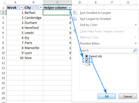
As the result, you have 0 in all even rows (because they are divided by 2 evenly without remainder) and 1 in all odd rows:

- Depending on whether you want to delete even or odd rows, filter out ones or zeros.
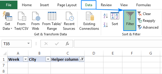
To have it done, select any cell in your Helper column, go to the Data tab > Sort and Filter group, and click the Filter button. The drop-down filter arrows will appear in all header cells. You click the arrow button in the Helper column and check one of the boxes:
- 0 to delete even rows
- 1 to delete odd rows
In this example, we are going to remove the rows with "0" values, so we filter them:

- Now that all "1" rows are hidden, select all the visible "0" rows, right-click the selection and click Delete Row:

- The above step has left you with an empty table, but don't worry, the "1" rows are still there. To make them visible again, simply remove auto-filter by clicking the Filter button again:

- The formula in column C recalculates for the remaining rows, but you don't need it anymore. You can now safely delete the Helper column:

As the result, only the even weeks are left in our worksheet, the odd weeks are gone!

Tip. If you'd like to move every other row to somewhere else rather than delete them altogether, first copy the filtered rows and paste them to a new location, and then delete the filtered rows.
How to delete alternate rows in Excel with VBA
If you are not willing to waste your time on a trivial task such as deleting every other row in your Excel worksheets, the following VBA macro can automate the process for you:
How to delete every other row in Excel using the macro
Insert the macro in your worksheet in the usual way via the Visual Basic Editor:
- Press Alt + F11 to open the Visual Basic for Applications window.
- On the top menu bar, click Insert > Module, and paste the above macro in the Module
- Press the F5 key to run the macro.
- A dialog will pop up and prompt you to select a range. Select your table and click OK:

Done! Every other row in the selected range is deleted:

How to delete every Nth row in Excel
For this task, we are going to expand the filtering technique that we've used to remove every other row. The difference is in the formula on which the filtering is based:
Where:
- m is the row number of the first cell with data minus 1
- n is the Nth row you want to delete
Let's say your data begins in row 2 and you want to delete every 3rd row. So, in your formula n equals 3, and m equals 1 (row 2 minus 1):
=MOD(ROW() - 1, 3)
If our data began in row 3, then m would equal 2 (row 3 minus 1), and so on. This correction is needed to sequentially number the rows, starting with the number 1.
What the formula does is divide a relative row number by 3 and return the remainder after division. In our case, it yields zero for every third row because every third number divides by 3 without remainder (3,6,9, etc.):

And now, you perform the already familiar steps to filter "0" rows:
- Select any cell in your table and click the Filter button on the Data
- Filter the Helper column to show only "0" values.
- Select all of the visible "0" rows, right-click and choose Delete Row from the context menu.
- Remove the filter and delete the Helper column.

In a similar fashion, you can delete every 4th, 5th or any other Nth row in Excel.
Tip. In cased you need to remove rows with irrelevant data, the following tutorial will come in helpful: How to delete rows based on cell value.
I thank you for reading and hope to see you on our blog again next week.
 by
by
6 comments
I have several Excel files that have data collected from automated test equipment. We got data at a rate about 10x higher than we need. The data files have 10x as many rows of data as we need.
I would like to modify the data files to keep every 10th row of data and delete all of the other rows.
I suspect there's a way to do this that is similar to what's presented in this article, but I'm not good enough at Excel to figure it out.
Any suggestions?
Hi! This formula will return TRUE on rows 1, 11, 21, etc.
=MOD(ROW(A1:A500),10)=1
I almost did it! (Delete 9 out of 10 rows).
I created a column called "Filter" in the first row. Then I used Mod(Row()-1,10 ) to get values 0 through 9 assigned sequentially to each row.
Then I used filtering so that every row labeled "0" was visible and all other rows (1 to 9) were hidden.
I'm using Excel on a Mac, so my UI is different from what you show, but with a bit of fiddling I figured it out.
The rows I want to remove were hidden, not deleted. So I followed your next step: Select the whole table of data and right click, then select "Delete Row".
When I did that I got a spinning beach ball for a few minutes, then Excel crashed.
The full data table has about 78,000 rows.
I restarted Excel and recovered the file.
In the recovered file, the results were still filtered (all "0" rows visible; and the "1 to 9" rows hidden). This time I selected the first two visible rows (not the entire data table), right clicked and selected "Delete Row". This deleted everything I selected. I.e., the "0" rows that I want to keep were deleted along with the "1 to 9" rows.
Any suggestions?
This worked, but in the opposite way that I intended. It keeps deleting the lines I want to keep and keeping the lines I want to get rid of. I've tried everything I could think of to make it work, I tried changing my row selections multiple times and I tried modifying the macro to Second row instead of First. It was the same result every time, and 3 hours later I'm exactly where I started.
I'm going to have to agree with the other commenter that this was an utter waste of time.
Hi Lauren,
We have updated the code, and now it works exactly as it should - removes every other row in the selection. In fact, there was just one wrong line, which caused so many problems... Sorry for that.
I just tried the sorting method with 1s and 0s. Infinitely easier. Wish I could have gotten a handle on using the macro, but unfortunately it wasn't meant to be.