Handy tools to manage text in Google Sheets

Change case in Google Sheets

Standard ways of changing the text case in Google Sheets include functions: LOWER, UPPER, PROPER. To use them, you will have to create a helper column, build formulas there, and reference your original column. Then somehow convert formula results to values and remove the original column.

Well, you don't need to do any of the above with our tool. It quickly changes the case in your Google Sheets in the original cells themselves.

You will find the tool in the the Text group > Modify:

To change case in your spreadsheet with this add-on, just select the range with your text and pick the way to modify data: turn everything into Sentence case., lower case or UPPER CASE, Capitalize Each Word (aka proper case), lower & or tOGGLE tEXT.

Once you're ready, press Modify and watch your original data change the case:

Replace symbols

If you import data from the web, you may find accented letters in your table like ß, Ö, or ç. The imported file may also contain different special characters: copyright signs (©), inverted question marks (¿), ampersands (&), and smart quotes (“ ”). These symbols may also be represented by their codes (often used on the web.)

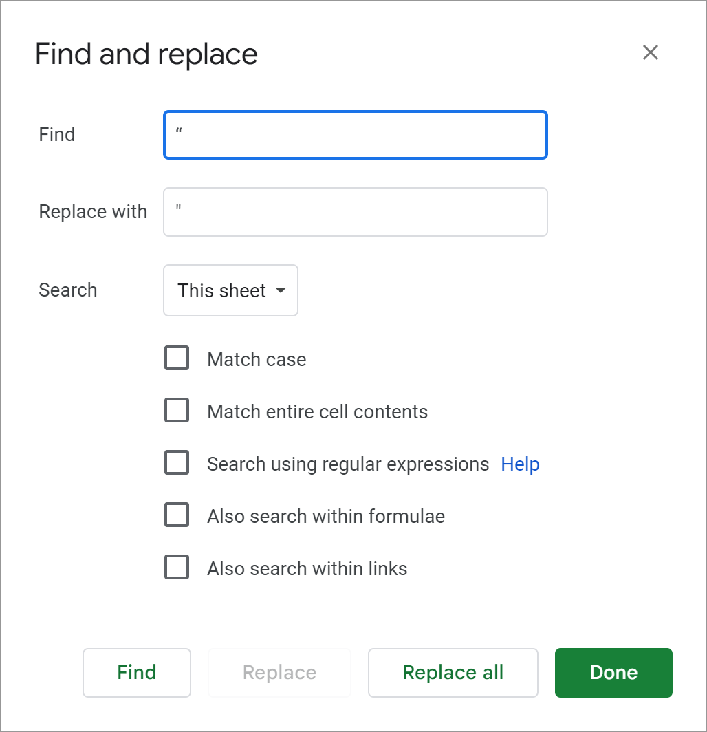
If you try to replace them using the standard Google Sheets Find and replace tool (Ctrl+H), prepare to go over the replacing process for each character. You will also have to enter symbols you want to see instead.

Our Replace symbols utility is much faster and easier to use. It scans the selected data range and automatically replaces all accented characters or codes with their corresponding standard symbols.

Here's also what you can do with codes and special characters using the same add-on:

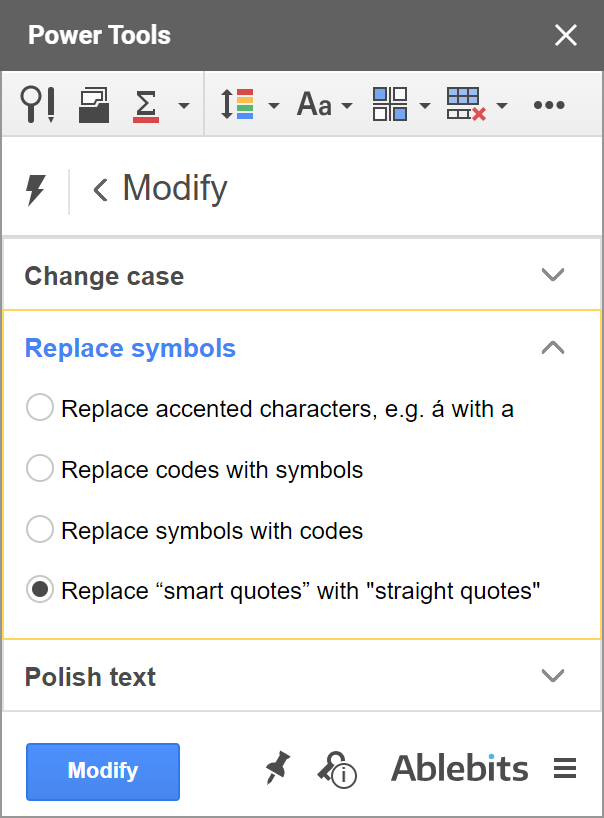
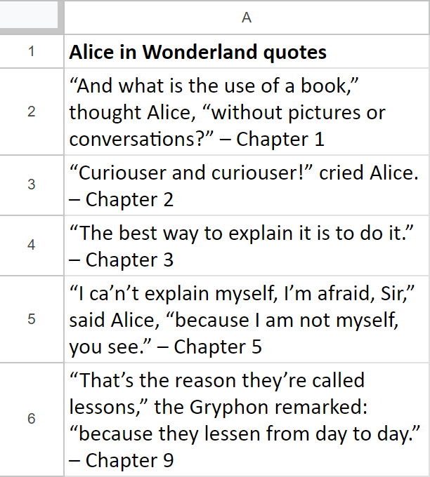
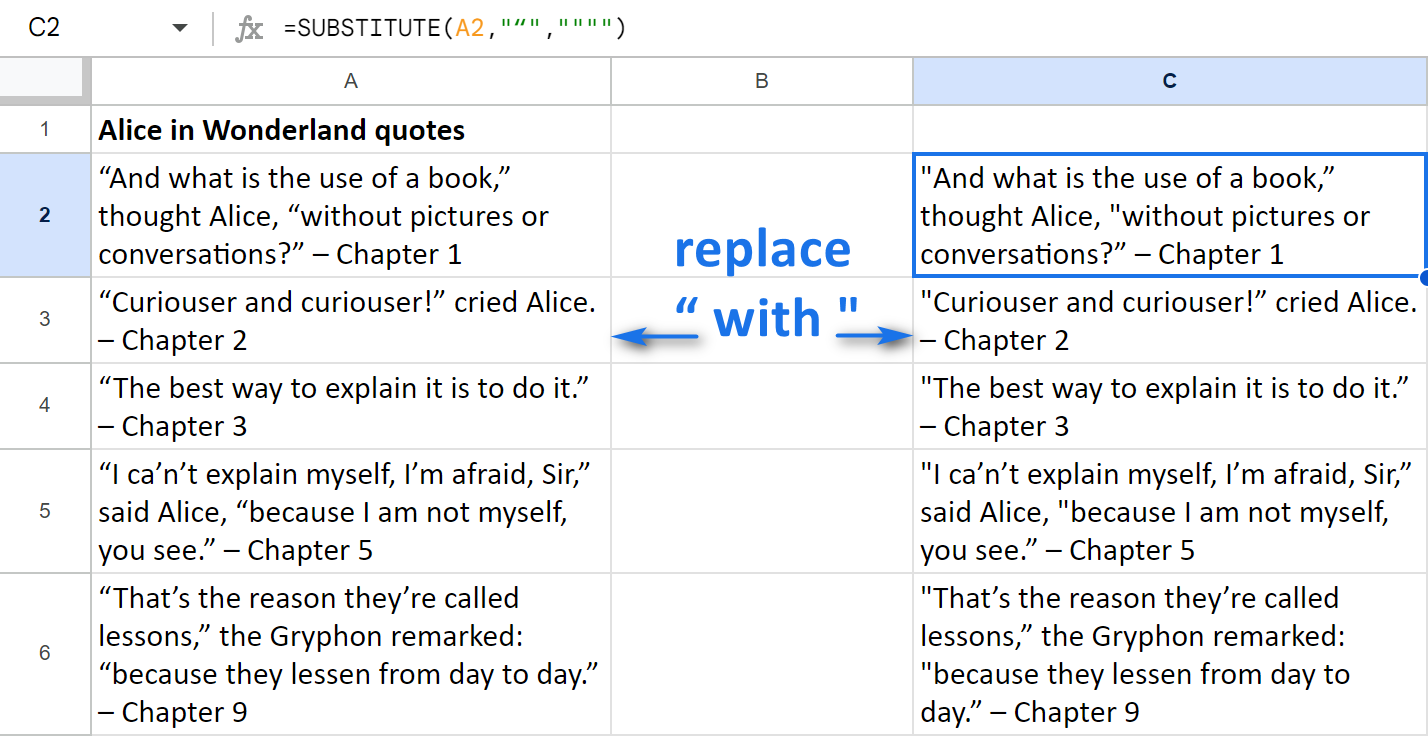
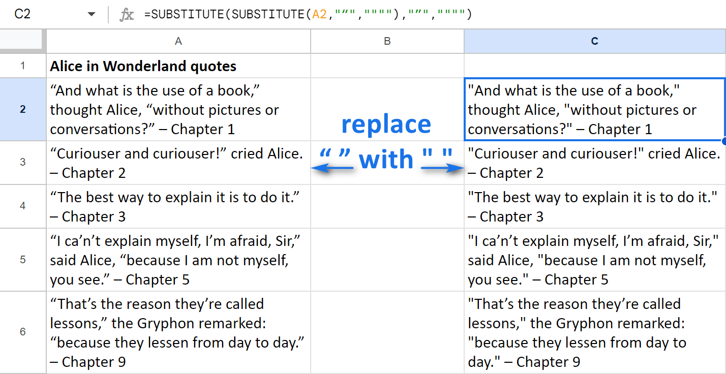
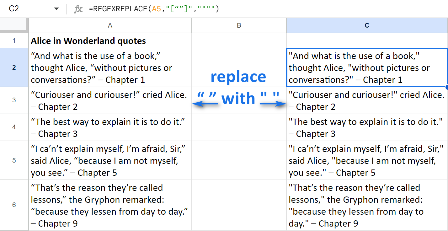
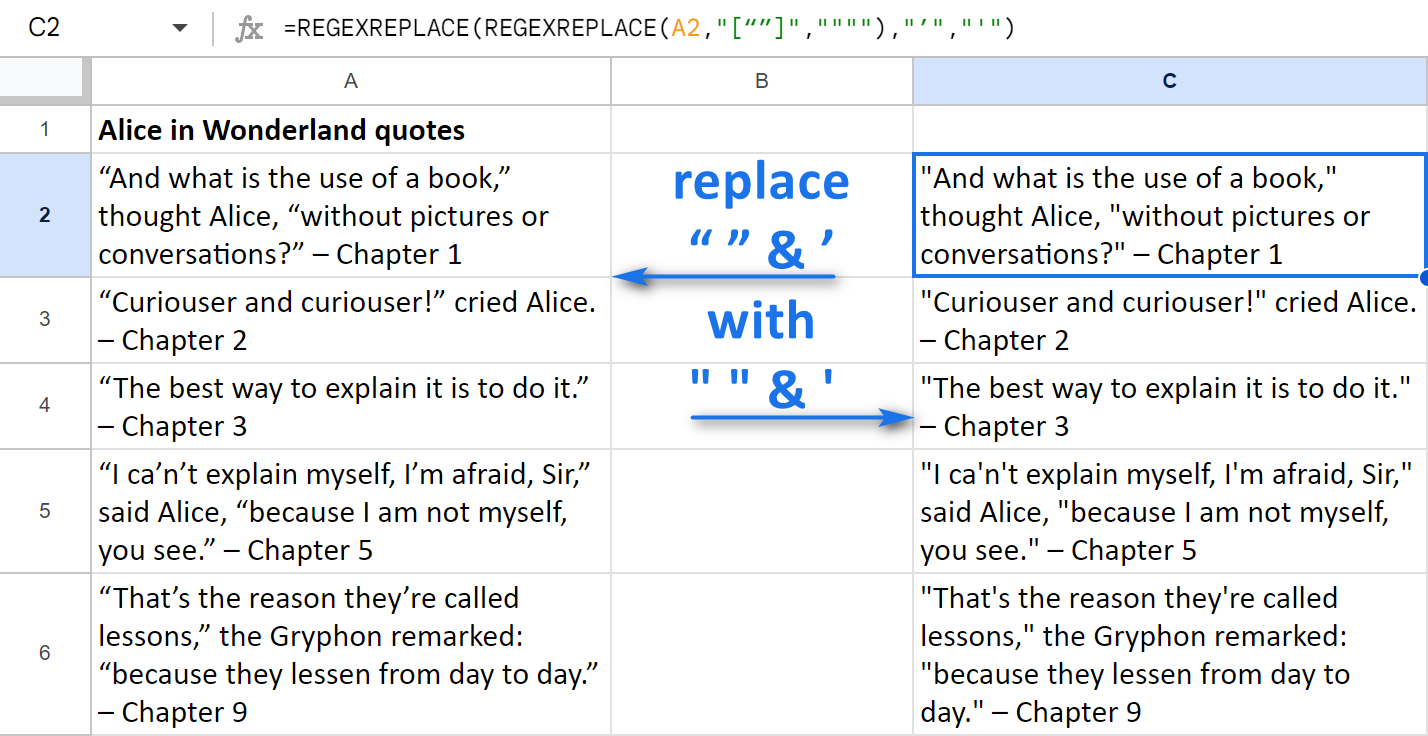
And here you can see how the Replace smart quotes with straight quotes tool works (currently for double-quotes only):

Polish text

If the modifications above are too much for your table, and you'd rather simply brush your Google Sheets text here and there, the add-on will help you automate this, too.

The Polish text tool looks through the range you select and does the following:

• removes white spaces if there are any
• adds space after punctuation marks if you forgot any
• applies sentence case to your cells

You are free to go with all three options at once or pick the one that suits your table best:

Insert special chars at the beginning / at the end

The first two options make it possible to add text at the beginning and at the end of all selected cells.

Let's say you'd like to supply your list of phone numbers with country codes. Since the code should precede the entire number, the task is to add numbers at the beginning of Google Sheets cells.

Just select the range with numbers, enter the desired country code into the corresponding field in the tool, and click Add:

Add text in Google Sheets before text / after text

The last three options of the tool let you insert characters depending on specific text in cells.

• You can add your text starting from the 3rd, 7th, 10th, etc. character in a cell with the option called After character number. I'm going to use this tool and insert area codes wrapped in brackets to the numbers from the previous example.

  There, area codes for the US and Canada numbers start from the 3d character: +12025550198. So I need to add a round bracket before it:
  

  Once added, the area codes end with the 6th character: +1(2025550198

  Thus, I add a closing bracket after it as well. Here's what I've got:
  

• You can also add text before or after specific text in cells.

  These options will help me make the phone numbers even more readable by adding spaces before and after the brackets:
  

But what if adding text in Google Sheets is not an option and you'd rather delete some excess chars and obsolete text? Well, we have the tools for this job as well.

Remove substrings or individual characters

This first tool gets rid of one or a few single characters and even Google Sheets substrings within the selected range. To be more exact, you can make it delete the following:

• all occurrences of one specific letter, number, or Google Sheets special character, e.g. 1 or +
• multiple single letters, numbers, or characters: e.g. 1 and +
• a specified sequence of characters — Google Sheets substring — or a few of such sets, e.g. +1 and/or +44

I'll take the same phone numbers from the previous example and remove all country codes and brackets at once with the tool:

Remove spaces and delimiters

The next utility for Google Sheets removes white spaces before, after, and within the text. If spaces are not welcome in your data at all, feel free to delete them completely:

The add-on also removes such special characters as commas, semicolons, and other delimiters (there's even a special checkbox for line breaks); non-printing characters (like line breaks), HTML entities (codes that are used instead of chars themselves), and HTML tags:

Remove chars by position

Sometimes though it is not the characters themselves that matter but their position in cells.

• In my example, there are extensions in phone numbers that take the same place — from the 12th to 14th character in each cell.

  I will use this position to remove the extensions from all numbers with the corresponding tool:
  

  Here's how the numbers transform in just a couple of clicks:
  

• You can clean up some amount of the first/last characters in cells in the same fashion. Just specify the exact number of extra symbols and the add-on won't keep you waiting.

  Have a look, the tool has removed country codes — the first 3 characters — from the phone numbers:
  

• If multiple cells contain the same text preceded or followed by unnecessary details, use the option Remove characters before/after text to cast them out.

  For instance, here's a list of clients with phone numbers and their countries in the same cells:
  

  Depending on the country, I select cells by groups and set the tool to remove everything before US, UK, and then CA. This is what I get as a result:
  

Remove empty rows and columns in Google Sheets

After various modifications to your data, you may notice empty rows and columns scattered all over your sheet. To delete them, the first way that comes to mind is to select each row while pressing Ctrl and then remove those blank lines via the context menu. And repeat the same for columns.

Besides, you may want to eliminate those unused columns and rows that remain outside your data. After all, they take up space and advance exceeding the limit for 5 million cells in a spreadsheet.

What's even more, you may need to do the same in all sheets within the file.

Unlike Google Sheets, our add-on removes all empty and unused rows and columns in one go. You don't even need to select any range or individual columns and rows.

Just open your sheet, access the Clear tool, select 5 checkboxes (or less, depending on your goal), click Clear, and there you have your neat tables in all sheets without any gaps:

Split by character

First, I'd like to demonstrate how to split text by characters or delimiters within cells.

You should select the data to split first, make sure the option to Split by characters is selected, and choose those separators that occur in your cells.

I don't check Space since I don't want to pull apart names. However, Comma and Line break will help me separate phone numbers and job titles. A also choose to replace my original column with the result (the checkbox at the very bottom of the add-on):

Split by position

As with adding text, the position of symbols in cells may be more significant than the occurrence of specific characters. Especially, if all cells are formatted in the same manner.

With the Split by position tool, you can choose a precise place at which records should be split:

I used this tool to separate country and area codes from the phone number itself:

All that remains now is to delete the original column and format those two new ones.

Split names

As I mentioned earlier, the standard tool of Google Sheets called Split text to columns merely drags words away from each other. If you use this tool for your names, there's a fair chance you'll get the columns where names, titles, and suffixes are mixed.

Our Split names tool will help you avoid that. It is intelligent enough to recognize first, last, and middle names; titles and salutations; post-nominals and suffixes. Thus, it doesn't just split the words. Depending on the name units, it puts them in the corresponding columns.

Moreover, you can pull, for example, only the first and last names no matter what other parts are there in cells. Watch this short video (1:45), the whole process takes literally just a few seconds: