If you've been following this blog for a while, you may remember QUERY function for Google Sheets. I mentioned it as a possible solution for a couple of cases. But those are far from enough to uncover its full potential. Today, it's high time we get to know this spreadsheets superhero properly. And guess what – one equally noteworthy tool will also be there :)
Did you know that Google Sheets QUERY function is considered to be the most powerful one in spreadsheets? Its peculiar syntax favours tens of different operations. Let's try and break its parts down to learn them once and for all, shall we?
Syntax of Google Sheets QUERY function
At first glance, Google Sheets QUERY is just another function with 1 optional and 2 required arguments:
- data is the range to process. Required. Everything is crystal clear here.
Note. Only one small reminder here established by Google: each column should contain one type of data: textual, or numeric, or boolean. If there are different types, QUERY will work with the one that occurs the most. Other types will be considered as empty cells. Strange, but keep that in mind.
- query is the way to process the data. Required. This is where all the fun begins. Google Sheets QUERY function uses a special language for this argument: Google Visualization API Query Language. It's written in a way similar to SQL. Basically, it's a set of special clauses (commands) used to tell the function what to do: select, group by, limit, etc.
Note. The entire argument must be enclosed in double-quotes. Values, in their turn, should be wrapped in quotation marks.
- headers is optional for when you need to indicate the number of header rows in your data. Omit the argument (as I do below), and Google Sheets QUERY will assume it based on the contents of your table.
Now let's dig deeper into the clauses and whatever they do.
Clauses used in Google Sheets QUERY formulas
Query language consists of 10 clauses. They may frighten at first glance, especially if you're not familiar with SQL. But I promise, once you get to know them, you will get a powerful spreadsheet weapon at your disposal.
I'm going to cover each clause and provide formula examples using this list of imaginary students and their paper subjects:
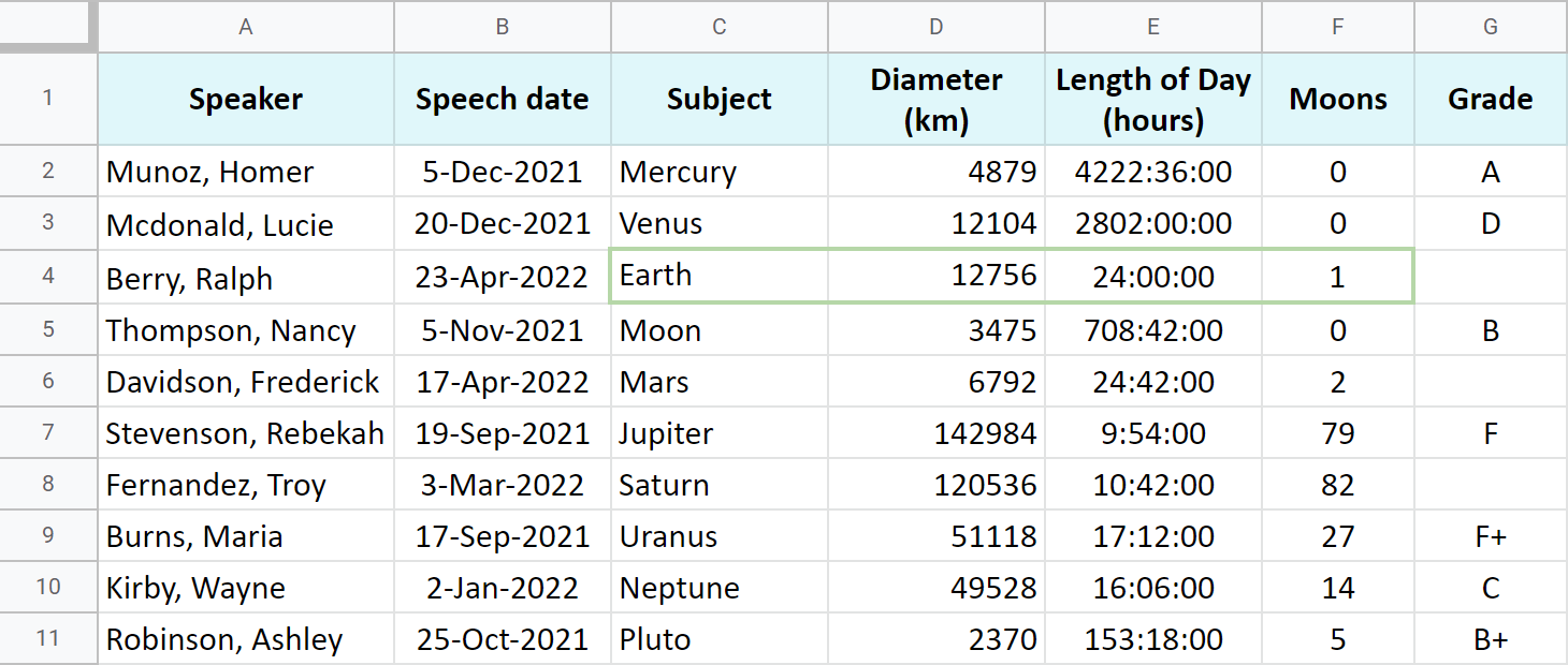
Yep, I'm one of those weirdos who think Pluto should be a planet :)
Tip. Several clauses can be used within one Google Sheets QUERY function. If you nest them all, make sure to follow the order of their appearance in this article.
Select (all or specific columns)
The very first clause – select – is used to tell what columns you need to return with Google Sheets QUERY from another sheet or table.
Example 1. Select all columns
To fetch each and every column, use select with an asterisk – select *
=QUERY(Papers!A1:G11,"select *")
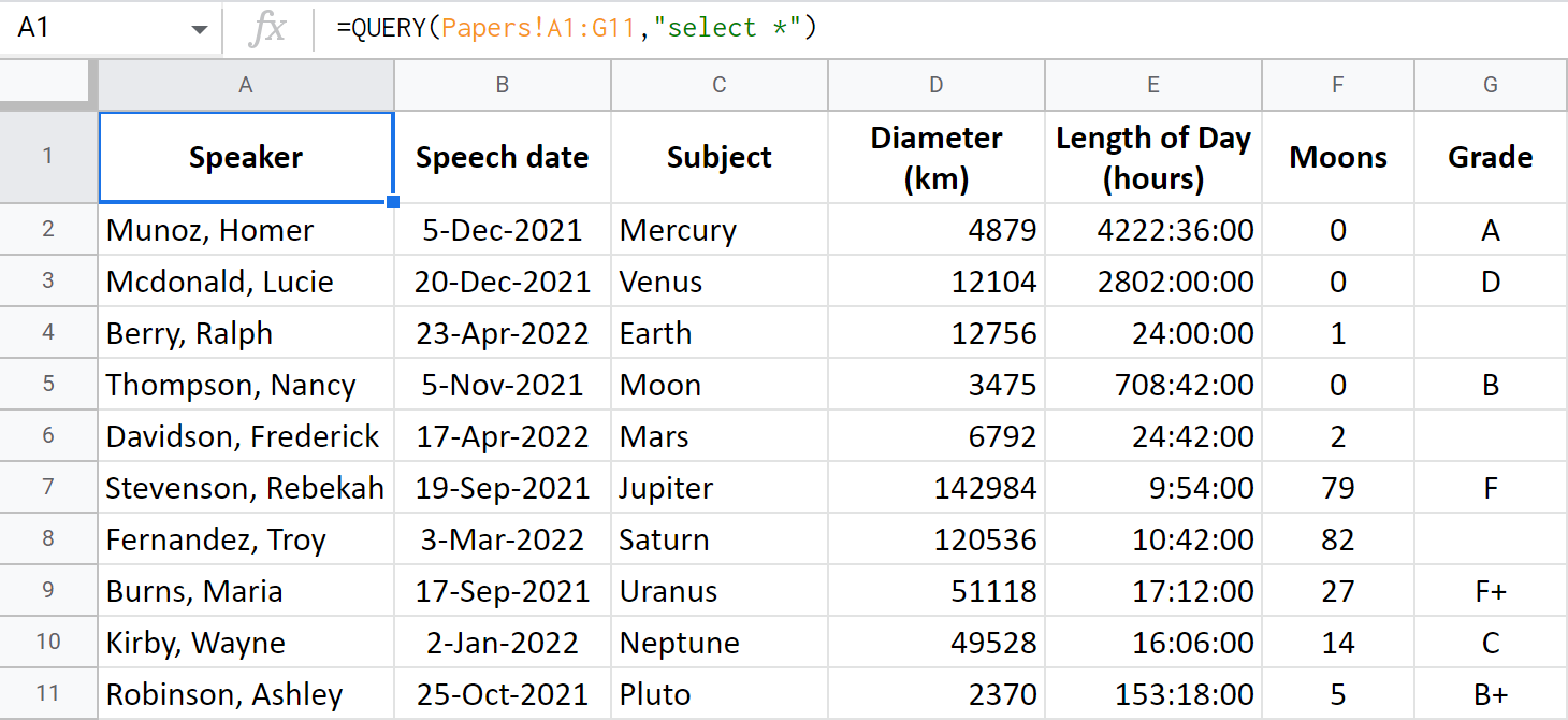
Tip. If you omit the select parameter, Google Sheets QUERY will return all columns by default:
=QUERY(Papers!A1:G11)
Example 2. Select specific columns
To pull only certain columns, list them after the select clause:
=QUERY(Papers!A1:G11, "select A,B,C")
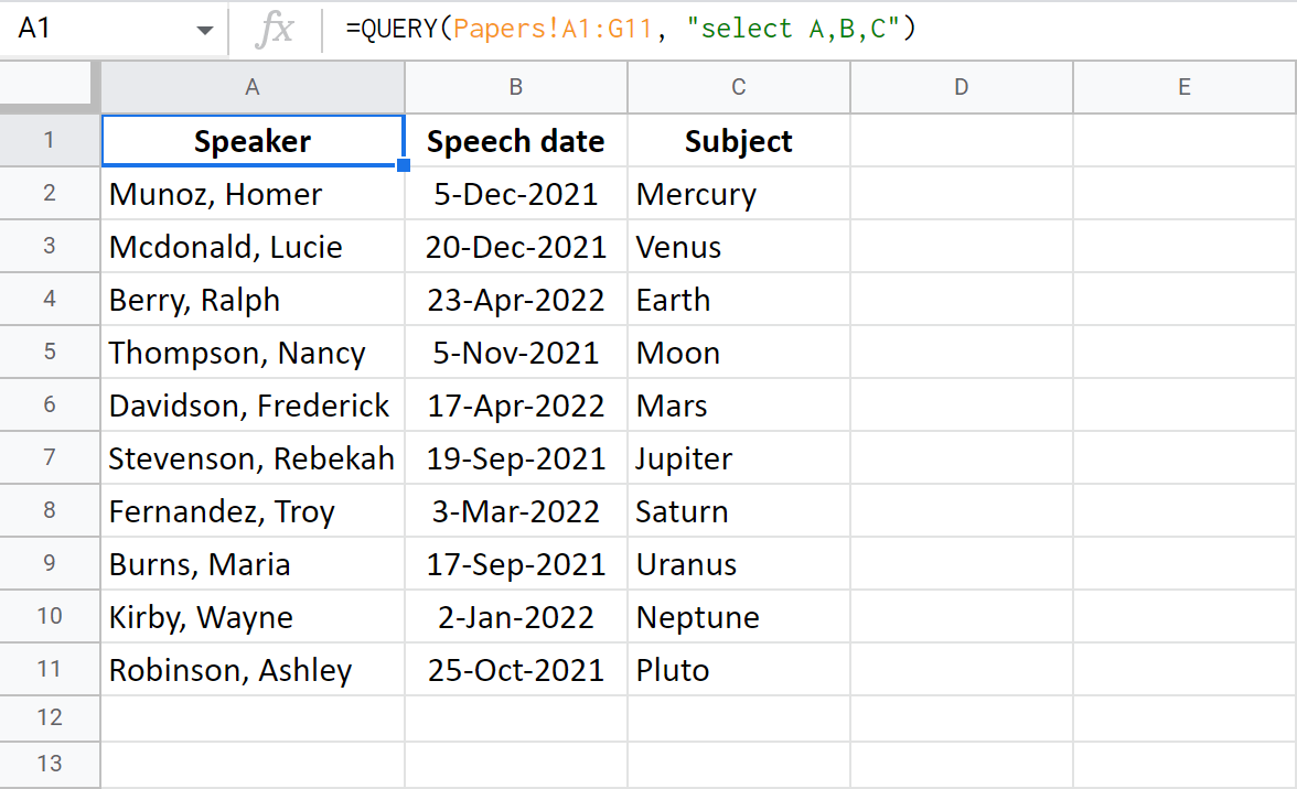
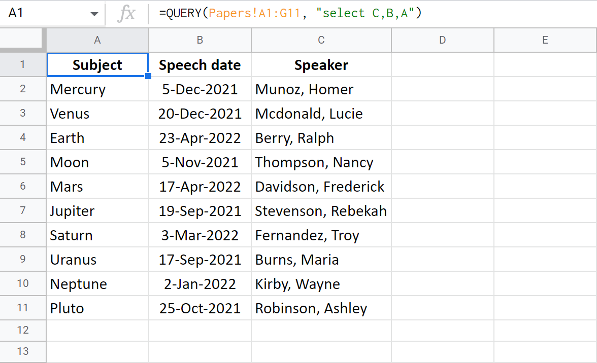
Tip. The columns of interest will be copied in the same order you mention them in the formula:
=QUERY(Papers!A1:G11, "select C,B,A")
Google Sheets QUERY – Where clause
Google Sheets QUERY where is used to set the conditions towards the data you want to get. In other words, it acts as a filter.
If you use this clause, QUERY function for Google Sheets will search columns for values that meet your conditions and fetch all matches back to you.
Tip. Where can function without the select clause.
As usual, to specify conditions, there are sets of special operators for you:
- simple comparison operators (for numeric values): =, <>, >, >=, <, <=
- complex comparison operators (for strings): contains, starts with, ends with, matches, != (doesn't match / doesn't equal to), like.
- logical operators to combine several conditions: and, or, not.
- operators for blank / not empty: is null, is not null.
Tip. If you're upset or worried about having to deal with such a huge number of operators again, we feel you. Our Filter and Extract Data will find all matches and build QUERY formulas in Google Sheets for you if necessary.
Let's see how these operators behave in formulas.
Example 1. Where with numbers
I will add where to my Google Sheets QUERY from above to get the info on those planets that have more than 10 moons:
=QUERY(Papers!A1:G11,"select A,B,C,F where F>=10")

Tip. I also mentioned column F to fetch just to make sure the criterion is met. But it's completely optional. You don't have to include columns with conditions into the result:
=QUERY(Papers!A1:G11,"select A,B,C where F>=10")
Example 2. Where with text strings
- I want to see all rows where the grade is either F or F+. I will use the contains operator for that:
=QUERY(Papers!A1:G11,"select A,B,C,G where G contains 'F'")
Note. Don't forget to surround your text with quotation marks.
- To get all rows with F only, just replace contains with an equal sign (=):
=QUERY(Papers!A1:G11,"select A,B,C,G where G='F'") - To check the papers that are yet to be delivered (where the grade is missing), check column G for blanks:
=QUERY(Papers!A1:G11,"select A,B,C,G where G is null'")
Example 3. Where with dates
Guess what: Google Sheets QUERY has even managed to tame dates!
Since spreadsheets store dates as serial numbers, usually, you have to resort to the help of special functions like DATE or DATEVALUE, YEAR, MONTH, TIME, etc.
But QUERY has found its way around dates. To enter them properly, simply type the word date and then add the date itself formatted as yyyy-mm-dd: date '2022-01-01'
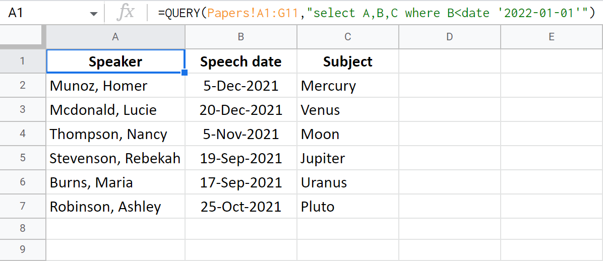
Here's my formula to get all rows with a Speech date before 1 Jan 2022:
=QUERY(Papers!A1:G11,"select A,B,C where B<date '2022-01-01'")
Example 4. Combine several conditions
To use a certain period of time as a criterion, you will need to combine two conditions.
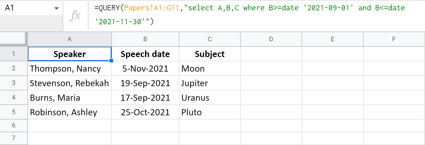
Let's try and retrieve those papers that were delivered in Autumn, 2019. The first criteria should be a date on or after 1 September 2021, the second — on or before 30 November 2021:
=QUERY(Papers!A1:G11,"select A,B,C where B>=date '2021-09-01' and B<=date '2021-11-30'")
Or, I can select papers based on these parameters:
- before 31 December 2021 (B<date '2021-12-31')
- have either A or A+ as a grade (G contains 'A')
- or B/B+ (G contains 'B')
=QUERY(Papers!A1:G11,"select A,B,C,G where B<date '2021-12-31' and G contains 'A' or G contains 'B'")

Tip. If your head is about to explode already, don't give up just yet. There's a tool that is perfectly capable of building all these formulas for you, no matter the number of criteria. Jump right to the end of the article to get to know it.
Google Sheets QUERY – Group By
Google Sheets QUERY group by command is used to concatenate rows. However, you should use some aggregate functions in order to summarize them.
Note. Group by must always follow the select clause.
Unfortunately, there's nothing to group in my table as there are no recurring values. So let me adjust it a bit.
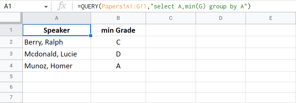
Suppose, all the papers are to be prepared by 3 students only. I can find the highest grade each student got. But since they are letters, it is the MIN function I should apply to column G:
=QUERY(Papers!A1:G11,"select A,min(G) group by A")
Note. If you don't use an aggregate function with any column in the select clause (column A in my example), you must duplicate them all in the group by clause.
Google Sheets QUERY – Pivot
Google Sheets QUERY pivot clause works the other way around, if I may say so. It transposes data from one column to a row with new columns, grouping other values accordingly.
For those of you dealing with dates, it can be a real discovery. You'll be able to get a quick glance at all the distinct years from that source column.
Note. When it comes to pivot, every column used in the select clause should be covered with an aggregate function. Else, it should be mentioned in the group by command following your pivot.
Remember, my table now mentions only 3 students. I'm going to make the function tell me how many reports each student made:
=QUERY(Papers!A1:G11,"select count(G) pivot A")

Google Sheets QUERY – Order By
This one is pretty easy :) It is used to sort the outcome by the values in certain columns.
Tip. All previous clauses are optional when using order by. I use select to return fewer columns for demonstration purposes.
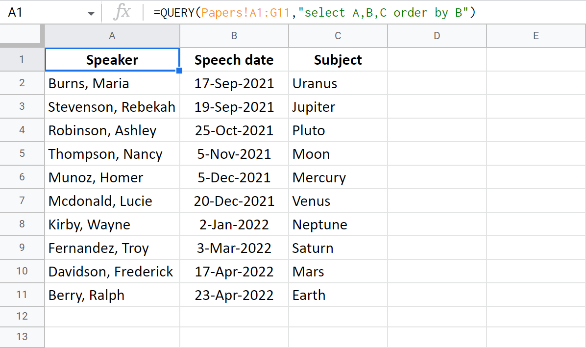
Let's go back to my original table and sort reports by speech date.
This next Google Sheets QUERY formula will get me columns A, B and C, but at the same time will sort them by date in column B:
=QUERY(Papers!A1:G11,"select A,B,C order by B")
Limit
What if I told you, you don't have to bring each and every row into the result? What if I told you that Google Sheets QUERY can pull only a certain amount of the first matches it finds?
Well, the limit clause is designed to help you with that. It limits the number of rows to return by the given number.
Tip. Feel free to use limit without other previous clauses.
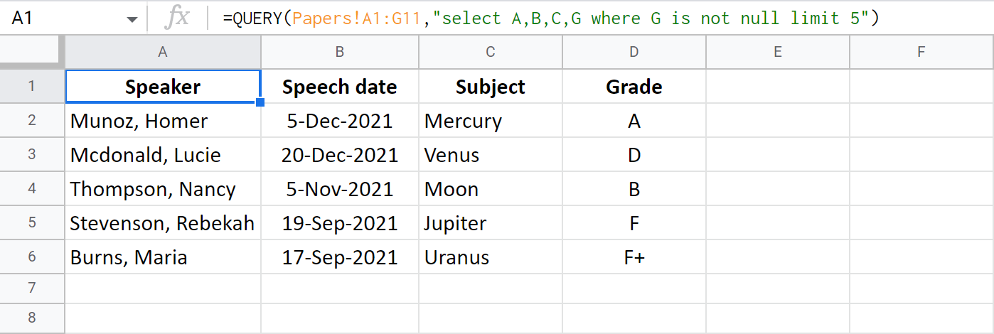
This formula will show the first 5 rows where the column with grades contains a mark (is not empty):
=QUERY(Papers!A1:G11,"select A,B,C,G where G is not null limit 5")
Offset
This clause is kind of opposite to the previous one. While limit gets you the number of rows you specify, offset skips them, retrieving the rest.
Tip. Offset also doesn't require any other clauses.
=QUERY(Papers!A1:G11,"select A,B,C,G where G is not null offset 5")

If you try and use both limit and offset, the following will happen:
- Offset will skip rows at the beginning.
- Limit will return a number of the following rows.
=QUERY(Papers!A1:G11,"select A,B,C,G where G is not null limit 3 offset 3")
Out of 11 rows of data (the first one is a header and QUERY function in Google Sheets does a nice job understanding that), offset skips the first 3 rows. Limit returns 3 next rows (starting from the 4th one):

Google Sheets QUERY – Label
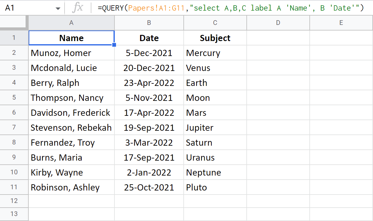
Google Sheets QUERY label command lets you change header names of the columns.
Tip. Other clauses are optional for label as well.
Put the label first, followed by the column ID and a new name. If you rename few columns, separate each new pair of column-label by a comma:
=QUERY(Papers!A1:G11,"select A,B,C label A 'Name', B 'Date'")
Format
The format clause makes it possible to alter the format of all values in a column. For that, you will need a pattern standing behind the desired format.
Tip. The format clause can also play solo in the Google Sheets QUERY.
=QUERY(Papers!A1:G11,"select A,B,C limit 3 format B 'mm-dd, yyyy, ddd'")

Tip. I mentioned some date formats for Google Sheets QUERY in this blog post. Other formats can be taken directly from spreadsheets: Format > Number > More Formats > Custom number format.
Options
This one is used to set some additional settings for the outcome data.
For example, such command as no_values will return formatted cells only.
The quickest way to build QUERY formulas – Filter and Extract Data
However powerful the QUERY function in Google Sheets is, it may require a learning curve to get ahold of. It's one thing to illustrate each clause separately on a small table, and completely another to try and build everything correctly with a few clauses and a much bigger table.
That's why we decided to dress Google Sheets QUERY up in a user-friendly interface and make it the add-on.
Why Filter and Extract Data is better than formulas?
Well, with the add-on there's absolutely no need to:
- figure out anything about those clauses. It's really easy to create lots of complex conditions in the add-on: as many as you need despite their order to fetch as many matches as you need.
Note. At the moment, the following clauses were incorporated into the tool: select, where, limit, and offset. If your task requires other clauses as well, please comment below – perhaps, you'll help us improve ;)
- know how to enter operators: just pick the one from a drop-down list.
- puzzle over the correct way to enter date and time. The add-on lets you enter them as you used to based on your spreadsheet locale.
Tip. There's always a hint available in the tool with examples of different data types.
As a bonus, you'll be able to:
- preview both the result and the formula
- make quick adjustments to your criteria
- select a place for the result
- insert the result as both QUERY formula or as values
I'm not kidding, see for yourself:
I hope you will give the add-on a chance and get it from Google Workspace Marketplace. Don't be shy and share your feedback, especially if there's something about it you don't like.
Also, feel free to check out its tutorial page or home page.
 by
by
152 comments
how to use mobile no column to pull data using query in google sheet ?
If you have any idea, can you please explain.
Hello Ramkumae,
I'm sorry, your question is not clear to me. What do you mean by 'mobile no column'?
how can I convert a column into text using Query+importrange formula in Select query, below is the formula details as its not working
=QUERY(IMPORTRANGE("","New Link Installations!A:AE"),"SELECT Col24, Text(Col26)",1)
Hello,
Sorry, I'm afraid I don't understand your task exactly. If you need to convert formulas to text, use the methods described here. If you need to convert dates, you may find the solution in this article.
Hello I am trying to write my function by selecting all of the values I have listed below and to not select 'Sold'. Can you see what is wrong with my formula?
"Select Col1, Col2, Col3, Col20, Col21 where Col2 contains 'Combine' or Col2 contains 'Truck' or Col2 contains 'ATV' or Col2 contains 'Sprayer' or Col2 contains 'Tractor' or Col2 contains 'Vehicles' and not Col3 contains 'Sold' "
Hello,
What error does your formula return? Try adding Order by as well to the end of your clause.
How would I correctly use the order by at the end of the clause?
Please see the example in the article. You just append it at the end and specify the column to order by.
If you're still having difficulties with your formula, for me to be able to help you, please share an editable copy of the spreadsheet that contains your formula with me: support@apps4gs.com. If you have confidential information there, you can replace it with some irrelevant data, just keep the format.
Note. We keep that Google account for file sharing only and don't monitor its Inbox. Please do not email there. Once you share the file, just confirm by replying to this comment.
How can I use group by when querying data from multiple sheets in the same googlesheet?
Hello Dennis,
Just as usual. The difference for multiple sheets is that you need to list the ranges from those sheets in the data argument, just like here.
I am doing a QUERY(IMPORTRANGE) from one sheet into another. I want the function to select rows from the source sheet where the values in the first and second imported rows equal values in two cell of the importing sheet. The value in the first cell, to match Col1, is a number.
The command =QUERY(IMPORTRANGE("18L1......","'RPCC Central Committee members'!C2:H12"),"select Col1,Col3,Col4,Col5,Col6 where Col1="&A4 &" "), it works fine to select rows where Col1 matches the value.
The value in the second cell, to match Col2, is a letter.
The command =QUERY(IMPORTRANGE("18L1.............","'RPCC Central Committee members'!C2:H12"),"select Col1,Col3,Col4,Col5,Col6 where Co21="&B4 &" ") produces the error: Error
Unable to parse query string for Function QUERY parameter 2: NO_COLUMN: C
What am I doing wrong?
Hello Conrad,
I can see 'where Co21' in the second formula. This doesn't look correct and should be Col2 if I understand the task correctly. Please fix this first and see if the error disappears.
Hello! Thank you for this great resource. I'm wondering if it's possible to to have the function SELECT particular columns based on the text in the column header, rather than the column number. So that maybe if a column in the source spreadsheet is shifted (but retains the same column header), the Query function would still get the same data.
Thanks!
Hello Nick,
I'm afraid QUERY doesn't take column headers as identifiers. It works only with column IDs as in the examples in the article.
Hello
is it possible to get output if one of C5 or C6 is empty?
=QUERY(Sheet1!A1:G30, "select * where D='"&C5&"' and C='"&C6&"' ")
Any help is greatly appreciated. Thank you!
Hello Haris,
Yes. Please check out Example 4. Combine several conditions in this part of the tutorial.
As for your formula, I believe you need to replace and with or to retrieve the data based on either of the conditions.
Hallo Natalia!
I'm trying to find get the correspondent value of said row, in column F, of the highest value in column E
currently i got this =query('Raw Data'!A2:G,"Select D,max(E),min(F),max(F) where D is not null group by D,E")
But i just want to keep the min value of F, and the correspondent value, of the max of E.
Is there any way to do this?
correction*
to keep the min value of F, and the correspondent value in F, of the max of E.
Hello Raul,
For me to be able to help you better, please share a small sample spreadsheet with us (support@apps4gs.com) with your data and the formula. Please also include the example of the result you expect to get. If you have confidential information there, you can replace it with some irrelevant data, just keep the format.
Note. We keep that Google account for file sharing only and don't monitor its Inbox. Please do not email there. Once you share the file, just confirm by replying to this comment.
I'll look into it and try to help.
Thanks for the reply
File shared!
Thank you for sharing the file, Raul.
I'm a bit confused however because your text description doesn't match the actual table and your actual formula. I'm not sure about the criteria you use to get the data.
Yet, from what I understand, I can suggest using QUERY to get the data based on columns A-D first, then enclose this into another QUERY as a range while adding other conditions for columns E-F. It'll look like =QUERY(QUERY(..., select ...), select ...)
Yes, i realized so mistakes were done with the file i had prior to my first comment, so i had it updated.
However i didn't know it was possible to place a query inside a query.
Thank you very much for the tip!
Best regards
- My main data tab has about 10 new rows added each day.
- My query tab has a query that pulls in certain things from each row, but still maintains each row and still adding about 10 new rows each day.
- To the right of my query, I have several columns that contain COUNTIF formulas, counting each time certain things happen in each row.
- The results from my COUNTIF formulas will feed into my Google Data Studio dashboard, and if I pull the formulas to the end of the page, zeros appear, which become a problem.
My question: Is it possible to have the COUNTIF formulas add new rows when the query adds new rows? Is there a way to turn my query into a table so the formulas fill in automatically, such as with excel tables? Or is there an alternate formula that I can pull to the bottom of the page and not get zeros?
Hi Amber,
There are a few things you can do:
Thank you Natalia. I've been looking for two days for how to order my query data, and this article solved it!
You're most welcome, Cameron, I'm glad the article helped!
Hi Natalia,
I have sheet1 and sheet2. On sheet1 there are two types of data below each other. type1 is manually data and type2 is query+importrange. On sheet2 I wanted to make a query based on sheet1 but not works with the query data. If I write manually in sheet1 its works on sheet2.
So in sheet1:
Col1 | Col2
KBL-001|EU
KBS-002|Magyar
LEO-001|Magyar
SEO-002|EU **//this is a query+importrange\\**
sheet2
=QUERY({'sheet1'!A2:B};"select Col1, Col2 where not Col1 contains 'seo' or not Col1 contains 'leo'")
Its works on LEO-001 but SEO-002 not. I tried importrange insted of 'sheet1'!A2:B too but does not work. In my opinion the problem is with the query based query. Is there any solution?
Thanks in advance
Hi Zsolt Gál,
I'm really sorry, I overlooked your comment. Do you still need a solution? If so, please consider sharing your spreadsheet along with your formula with us (support@apps4gs.com). If you have confidential information there, you can replace it with some irrelevant data, just keep the format.
Note. We keep that Google account for file sharing only and don't monitor its Inbox. Please do not email there. Once you share the file, just confirm by replying to this comment.
I'll look into the problem and try to find a solution.
Hi, can you please help me to understand how to do better in this case, I want to add different condititions for my imported data, but once I delete the value from one of sell, the origin files import all field to the current file.
=query({IMPORTRANGE("1c6ihzJjzD_Nhbz5rB1s0485PS98V-Q4bfVAiIon5vSA","MC2!A11:S5000")},
"select Col19, Col1, Col2, Col3, Col5, Col6, Col7, Col8, Col9, Col10, Col11, Col12, Col13, Col14, Col15, Col18
where (Col8 contains '"&B2&"')
or (Col8 contains '"&C2&"')
or (Col8 contains '"&D2&"')
and (Col8 is not null)
and (Col5 is not null)
order by Col6 asc,
Col10 asc",0)
https://docs.google.com/spreadsheets/d/1gYMouKgMmcD4g27dZnR5M2pQwxMEHOhM8xJunr7CHKg/edit?usp=sharing
Hi Ann,
Thank you for sharing the file. Unfortunately, it's hard to tell what's happening because I have no editing access to your spreadsheet. I tried to reproduce the problem on dummy data on my side but everything works correctly there. Perhaps, you could share an editable copy of your file with me? You can share it directly with support@apps4gs.com
Also, please specify if you delete the value from the origin file or from this spreadsheet. Which value do you remove exactly? What happens with the data returned by QUERY once you remove that value? You can also add more sheets to your file featuring your data before/after removing the value.
Thanks!
I just shared the file with you.
The issue is
if I delete - Select a state 3 MN (CELL D2) - then there is a mess with the imported data.
I just want to give a condition, if one of my B2, C2 or D2 is empty
import only the rows from my query which contains one of them
In my case, if D2 is empty the formula is importing all empty spaces from my main spreadsheet
Thank you for editing permissions and additional example sheets!
I duplicated your sheets without formulas and entered the correct QUERY there. It's the same formula on both sheets, looks like what you need :)
=QUERY({IMPORTRANGE(Abb!F3,"MC2!A11:S5000")},
"select Col19, Col1, Col2, Col3, Col5, Col6, Col7, Col8, Col9, Col10, Col11, Col12, Col13, Col14, Col15, Col18
where (Col8 contains '"&IF(B2 = "",false, B2)&"')
or (Col8 contains '"&IF(C2 = "",false, C2)&"')
or (Col8 contains '"&IF(D2 = "",false, D2)&"')
and (Col8 is not null)
and (Col5 is not null)
order by Col6 asc,
Col10 asc",0)
Hi Natalia,
Thank you for sharing this, I am building a dashboard using query, I would like to know if there is a way to insert a sumproduct function within query in google sheet, if so, please let me know how, that is one step that I need to complete my dashboard, appreciate it!
All the best!
Hi Gail,
For me to be able to help you better, please share a small sample spreadsheet with us (support@apps4gs.com) with 2 sheets: (1) a copy of your source data with the QUERY (2) the result you expect to get. The result sheet is of great importance as it gives us a better understanding than any text description.
Note. We keep that Google account for file sharing only and don't monitor its Inbox. Please do not email there. Once you share the file, just confirm by replying to this comment.
I'll look into your data and try to find a solution.
Hi Natalia,
Apologies for replying late, I was able to solve the problem; thank you so much for the support
Hi Gail,
Thank you for replying! Glad to know you were able to solve your task :)
I need Two Condition (1) IF I do not select anything from the Drop Down still My Entire Data gets reflected (2) and if I select A particular name from the Drop Down List the the Data Related to that Client gets extracted.
Please assist.
Hello Sumit,
please consider sharing an editable copy of your spreadsheet with us (support@apps4gs.com) with 2 sheets: (1) your source data, (2) the result you want to get.
Note. We keep that Google account for file sharing only and don't monitor its Inbox. Please do not email there. Once you share the file, just confirm by replying to this comment.
If you have confidential information there, you can replace it with some irrelevant data, just keep the format. I'll look into it and try to help.
Hello!
I want to generate a quotation from múltiple variables from a list (Gender, Age, Product, etc). In order to do it I need a specific rate from another table and I am using the Query function as you shown but need to include a Vlookup function into the query, is it posible?
This is where I am.
=QUERY(Rates!A3:AN215,"SELECT * WHERE ((lower(A) = lower('"&Cotizador!D14&"'))) AND ((lower(B) = lower('"&Cotizador!D8&"'))) AND ((lower(C) = lower('"&Cotizador!D12&"'))) AND ((D = "&Cotizador!D10&"))", true)
After bringing the results given those criterias, I need then it to go and pick the rate from a specific column where the header is the age so after I get that value, calculate the formula for the quotation.
Thanks!
Hello Marino,
I'm sorry but your task is not really clear. For me to be able to help you better, please share a small sample spreadsheet with us (support@apps4gs.com) with 2 sheets: (1) a copy of your source data (2) the result you expect to get. The result sheet is of great importance as it gives us a better understanding than any text description.
Note. We keep that Google account for file sharing only and don't monitor its Inbox. Please do not email there. Once you share the file, just confirm by replying to this comment.
I'll look into your data and try to find a solution.
Hello,
I am trying to write a query that only returns the columns where the matching row value is greater than 0.
Here is the part that works:
query('Sub Cap Mat Requirements'!$A$1:$P$422,"Select F, G, H, I, J, K, L, M WHERE A = '"&$C$3&"' AND
please could you help me finish it!
In one example I don't want column M returned as the row value is 0, but if I change the value in C3, then it may be column J that's 0 so that would be the column I would want omitted from the results.
Thanks in advance!
Hello Kahl,
I'm afraid your formula won't work. Here's another one for you to try:
=QUERY({A1:P422},"select "&ArrayFormula(JOIN(",","Col"&QUERY({TRANSPOSE({QUERY({A1:P422},"select * where Col1 = '"&C3&"' limit 1",1);ARRAYFORMULA(COLUMN(A1:P1)-1)})},"Select Col3 where Col2 <> 0",1)+1)),1)
Thank you!???
Does anyone know how to =Query from multiple sheets?
Hello Aekaterini,
I believe you will find the answer to your question here:
Google Sheets QUERY to import ranges from multiple sheets
What a gold mine, thank you!!
Is it possible to search by column and row? I'm having trouble formatting it.
For instance: "SELECT * WHERE Col1='Revenue' AND Row1='2022' "
Thank you for your feedback, Ohad!
I'm sorry I don't really understand what this condition should return. Please share a small sample spreadsheet with us (support@apps4gs.com) with 2 sheets: (1) a copy of your source data (2) the result you expect to get (the result sheet is of great importance and often gives us a better understanding than any text description). I kindly ask you to shorten the tables to 10-20 rows.
Note. We keep that Google account for file sharing only and don't monitor its Inbox. Please do not email there. Once you share the file, just confirm by replying to this comment.
I'll look into it.
Is there a way to limit the number of columns in the query pivot? I suppose the follow up to that would also be ordering it by the total of the pivoted columns
Hello George,
To return a particular number of columns, just specify those columns in the "select" command. Please see Example 2 in this part of the article.
Ordering is also possible and described here.
How to use this query formula in excel to pull multiple column data from one tab to another
Hello Shubh,
Sorry but the QUERY function doesn't exist in Excel. Please look through this blog post to see what other functions exist in Google Sheets only.
Hi,
I would like to return values from a different google sheet with details below:
=query(IMPORTRANGE(B7,"UCaaS!B:B"),"Select * where B contains 'Citrix'")
I am getting this error: Unable to parse query string for Function QUERY parameter 2: NO_COLUMN: B
Appreciate your help on this. Thank you.
Hi Fer,
Try replacing 'B' with 'Col2':
'where Col2 contains'
While getting data from different sheets in a main sheet through query function, it shows error"In ARRAY_LITERAL, an Array Literal was missing values for one or more rows." when takes range A9:O and when I takes A8:O its working but it is taking headwer of all and I want only data.
Query is :
={query(Ajmer!A9:O,"Select A,B,C,G,O where O='"&B1&"'");query(Sikar!A9:O,"Select A,B,C,G,O where O='"&B1&"'");query(Jhotwara!A9:O,"Select A,B,C,G,O where O='"&B1&"'");query(Chaksu!A9:O,"Select A,B,C,G,O where O='"&B1&"'");query(Bassi!A9:O,"Select A,B,C,G,O where O='"&B1&"'");query(Bijaynagar!A9:O,"Select A,B,C,G,O where O='"&B1&"'");query(Bhilwara!A9:O,"Select A,B,C,G,O where O='"&B1&"'");query(Chomu!A9:O,"Select A,B,C,G,O where O='"&B1&"'");query(Chittorgarh!A9:O,"Select A,B,C,G,O where O='"&B1&"'")}
Hello Chandra,
This error usually occurs whenever there is a blank sheet or a sheet with only a header row among your original tables. Can you check that?
Hi,
We are using the query function to get data from a Master Sheet(let's say SheetA) and show it another Sheet (SheetB). We are facing issues due to the high number of people (~1000) accessing the sheets. Is there a way to identify the number of active connections made by query function so that we can alert the users in some way? Please suggest if there is a better workaround to navigate this number of users problem?
Thanks
Hi Sarathy,
Sorry, could you specify what you mean by 'active connections made by query function'?
Can I overwrite data that has been queried?
I have my query set to pull based on date, I then need to overwrite the cell that contains "yes". Can this be set up without deleting all my data?
Hello Rebeca,
Everything returned by QUERY is part of the formula. To overwrite its part, you need to convert the entire formula into values first.
Is there a limit to the select range of rows or cells it will work with?
For example if I used this QUERY(Calculations!A2:T1500, "select A, B, C where (S>0)", 1)
It'll return one line of data.
If the I used this QUERY(Calculations!A2:T1200, "select A, B, C where (S>0)", 1) Note its 1200 rows not 1500 it will return all the lines of data.
Thanks
Hello Max,
The formula always works within the range you indicate. If you limit it by 1200 rows, it won't look at rows 1201 and further.
In case you need an unlimited number of rows (include all future rows in the result), you need to use a reference like this: Calculations!A2:T
Hello,
I have a query function pulling specific lines from one tab to separate tabs based on information provided in specific columns (info coming in from a connected google form). The query was working well and then suddenly started filtering all of the information into a single line in each tab. Examples of the queries used are:
=query('Form Responses 1'!A2:BJ, "Select*where C='Leadership / Dr. J' and L='Yes'")
=query('Form Responses 1'!A2:BJ, "Select*where C='Green Energy - Dr. Smith' and L='Yes'")
The problem persists even when I try to simplify the query:
=query('Form Responses 1'!A2:BJ, "Select*where C='Leadership / Dr. J'")
Any support in figuring out why the queries stopped sorting and how to get them up and running again would be very much appreciated.
Thanks!
Hello Marie,
For me to be able to help you, please consider sharing an editable copy of your spreadsheet with us (support@apps4gs.com). If you have confidential information there, you can replace it with some irrelevant data, just keep the format. I'll look into it.
Note. We keep that Google account for file sharing only and don't monitor its Inbox. Please do not email there. Once you share the file, just confirm by replying to this comment.
Hi!
I hope you're doing well.
I want to use the query function to display a data set where the query looks like
=QUERY('Student Data Dump'!A2:K, "SELECT * where F='International Business Management - Logistics System (B999)'")
However rather than typing the F column manually, I want to assign it to a drop down cell. So that I could select what data to display based on what the A2 cell has.
I tried the same with =QUERY('Student Data Dump'!A2:K, "SELECT * where F= IBM-LS!A2 ") but that doesn't work.
Could you help me out with the same? Thanks!
The link to the sheet is https://docs.google.com/spreadsheets/d/1NIPzSZ1nCNTgekDN5-40NLAPxKg6lszFpVJFMFIFHVM/edit#gid=192360295
Hi Nitish,
Your sample spreadsheet is locked from editing. The correct way to reference other cells in QUERY formulas is like this:
=QUERY('Student Data Dump'!A2:K, "select * where F = '"&'IBM-LS'!A2&"'")
Hello, I have a query where I have the top 10, but am trying to find the next 10 now
=query(A:BA), "SELECT Col10, sum(Col51)/1000 WHERE Col9='XXX' Group by Col10 Order by sum(Col51)/1000 desc limit 10 LABEL Col10 '', sum(Col51)/1000 ' '",-1)
Offset only removes the first 10 rows from the original data set, not from the grouping, so was hoping to group desc next 10 if that's possible?
Thanks!
Hello Lola,
Offset is exactly the clause that you'd use to find 'the next 10'. Can you please share an editable copy of your file with us (support@apps4gs.com) where you used the formula and it didn't work? Also, please include the example of the result you'd like to get, it will give us the exact picture of your task. Thank you.
Hello,
I have 15 columns with Group tag as header and containing lists of names.
Some names appears in different columns / Group tags.
How can I display in a single cell the different columns headers / Group tags where a specific name is appearing?
Thank you in advance,
Hello Pierre,
For me to be able to help you, please share a small sample spreadsheet with us (support@apps4gs.com) with 2 sheets: (1) an example of your source data (if you have confidential information there, you can replace it with some irrelevant data, just keep the format) (2) the result you expect to get (the result sheet is of great importance and often gives us a better understanding than any text description). I kindly ask you to shorten the tables to 10-20 rows.
Note. We keep that Google account for file sharing only and don't monitor its Inbox. Please do not email there. Once you share the file, just confirm by replying to this comment.
I'll look into it.
Hello Natalia,
The file has been shared with you.
Thank you in advance once again,
Pierre
Hello Pierre,
Thank you, I've got the file. I'll look into it as soon as possible and try to come up with a solution.
Hello Pierre,
Please look at column N in your spreadsheet. I placed the formula to N2 and copied it down:
=TEXTJOIN(", ",TRUE,QUERY({QUERY({TRANSPOSE(QUERY($B$1:$J$10,"select *",1))},"select Col"&TEXTJOIN(",Col",TRUE,ArrayFormula(ROW(INDIRECT("1:"&ROWS({TRANSPOSE(QUERY($B$1:$J$10,"select *",1))})))))&" where Col"&TEXTJOIN("='"&M2&"' or Col",TRUE,ArrayFormula(ROW(INDIRECT("1:"&ROWS({TRANSPOSE(QUERY($B$1:$J$10,"select *",1))})))))&"='"&M2&"'",0)},"select Col1",0))
Thank you !
You're most welcome! :)
I am using Query in a google sheet , but all the results are coming together in the 1st row only and from the 2nd row it is coming properly .
For example : Data should be like..
Col 1 Col 2 Col 3
A B. C
D. E. F
But the Data is coming like after using Query function :
Col 1. Col 2. Col 3
A D. B E C F
D. E. F
Hello Madhusmita,
What formula do you use exactly? Please provide it here.
How can I add an order function to this query where it will sort both sets of data together in one list? Basically I want to pull two sets of data then have both sets ordered together in one long list.
={query('Reg Data'!A:AA,"Select F, E, H, K, U, R, V, X, G, Y, AA WHERE S='US History A'",0); query('Reg Data'!A:AA,"Select F, E, H, K, U, R, V, X, G, Z, AA WHERE T='US History A'",0)}
I want to sort the entire list using this: Order by R, F, E
Thank you for your help.
Hello Neal,
By adding the 'order by' clause to each QUERY, you will sort each range individually.
To sort the entire result, you need to wrap QUERY in the SORT function:
=SORT({QUERY('Reg Data'!A:AA,"select F,E,H,K,U,R,V,X,G,Y,AA where S='US History A'",0); QUERY('Reg Data'!A:AA,"select F,E,H,K,U,R,V,X,G,Z,AA where T='US History A'",0)},5,TRUE,6,TRUE,18,TRUE)
I would like to figure out how to search by numbers. I have =QUERY(' Install PO Log'!B2:P,"SELECT * WHERE P = '72'",1) and I basically have jobs that are all assigned their specific numbers and I want to group the jobs by the numbers rather than by their name in order to simplify some other things for me. Is that possible? I can't figure it out, It only seems to work when I search by letters.
For Example:
This is my job list:
Mcdonalds 1
Arbys 2
Wendys 3
Arbys 2
Arbys 2
Mcdonalds 1
I want to group them by searching by "2" instead of "Arbys" is that possible?
Hello Jacob,
When searching for numbers, do no put them into single quotes:
=QUERY('Install PO Log'!B2:P,"SELECT * WHERE P=72",1)
Only text strings should be wrapped in quotes in Google Sheets formulas.
You just solved an issue I had been trying to solve for 6+ hours thank you so much!
My next question is how I select certain columns. I have Columns A-P but I only need columns B,C,D,F,G,H,I,J,M,N,P. Right now, I have to hide the columns I don't need but that's very time-consuming when I have hundreds of these formulas to do. Is there any way to throw those specific columns into the formula so only they show? Below is the formula I am using now and I would just like to only use specific columns.
=QUERY(' Install PO Log'!B2:P,"SELECT * WHERE P = 53",1)
Just list those columns instead of * in the formula :)
=QUERY('Install PO Log'!B2:P,"SELECT B,C,D,F,G,H,I,J,M,N,P WHERE P = 53",1)
BTW, I explained it in this part of the blog post: Select (all or specific columns)
I would like to type a date into one cell... and have a query pull a column from another page that has dates in the top row (i'd like to search for the date here). Is this possible, and if so, what would the formula look like?
Hi James,
For me to be able to help you better, please share a small sample spreadsheet with us (support@apps4gs.com) with 2 sheets: (1) a sample of your data (2) the result you expect to get. I kindly ask you to shorten the tables to 10-20 rows. If you have confidential information there, you can replace it with some irrelevant data, just keep the format. I'll look into it.
Note. We keep that Google account for file sharing only and don't monitor its Inbox. Please do not email there. Once you share the file, just confirm by replying to this comment.
Hi, i have an issue and need help please :)
When both query have numbers it's working but when one doesn't find a result i have N/A error, i can't find a way to solve that even with a "ifna"
=IF(isblank(B9),,{QUERY(Dividendes_TFSA!$B$8:$F$55,"select F where B='"&B9&"' and C like '%March%'")+QUERY(Dividendes_RRSP!$B$9:$H$55,"select G where B='"&B9&"' and C like '%March%'")})
Thank you very much.
Hi Angelique,
You can wrap each QUERY in IFNA so they return 0 if there's no numeric result, like this:
=IF(ISBLANK(B9),"",IFNA(QUERY(A2:B5,"select B where B="&B9,0),0) + IFNA(QUERY(A6:B10,"select B where B="&B9,0),0))
Hello, I am wanting to pull columns from a named range based on a cell value in the sheet I'm pulling the info into but I can't seem to figure out how to do it.
I want columns D, O and P from the named range All2021Regos where C = my current spreadsheets C2.
=Query(All2021Regos,"select D,O,P Where C=C2")
=Query(All2021Regos,"select D,O,P Where C='Attendance Sheet auto'!C2",)
I was hoping for something like this, but with a named range, and with having a cell determine the value rather than having it in the formula.
=QUERY(IMPORTRANGE("insert_url","Range"),"Select Col1, Col2 Where Col4='Value'")
Any help would defs be appreciated.
Hello Sam,
You can try this one:
=QUERY(All2021Regos,"select D,O,P where C='Value'")
Or, if you'd like to reference a cell, you need to let QUERY know that it's a reference, not a column name (I add 1 at the end, so it sees the header row):
=QUERY(All2021Regos,"select D,O,P where C='"&C2&"'", 1)
Hello, thanks for taking the time to write great blogs and helping us all so much.
My issue is I am using query to select figures from a couple of columns (that are created each day and so generally differ in length) which relate to volumes of sales of different products. I can exclude the top row from being sorted alphabetically but the 'Totals' row at the bottom is swept up and included.
If I call it 'zz Total' obviously it stays down where I want it to be but that's horrible - is there a way to exclude the final line from being included in the query search?
Hello Nick,
Thank you for the feedback! :)
You can make the formula ignore the first and the last rows using the ArrayFormula and OFFSET functions respectively for the 'limit' command. Here's an example:
=QUERY({Sheet10!A1:E}, "select * limit " &ArrayFormula(max(if(len(Sheet10!A1:E), ROW(Sheet10!A1:E), )))-2 & " OFFSET 1", 0)
If you're not sure how to incorporate that into your own QUERY, please provide your exact formula here.
Hi Natalia,
I was hoping you can assist!
Column H I J is where my datas are and I need to return the data if what I type in Column G matches column H — what is the best way to go about this?
Hi Cassie,
I believe the IF function will help you with the task :)
Hi Natalia, How can i find rows in a column(that has sentences as values) that dont contain a particular word?
Hi Saumittra,
Supposing it's a column A, the following formula will do the trick:
=QUERY(A:A,"select * where not A contains 'particular_word'")
is there a way to return the query results with bordered cells. I mean make cells that have results with borderes
Hello Hassan,
I'm sorry but standard Google Sheets formulas don't pull the formatting of the processed cells.
Hi
Great article, but I'm stuck and wondered if you can help, I'm Trying to get a (Where) query to return columns from sheet1 into sheet2 where the criteria to meet is in col1 in sheet2!
An example from your article is 1 below, but I'm trying to achieve 2?
1) =QUERY(Sheet1!A1:G11,"select A,B,C,F where F>=10")
2) =QUERY(Sheet1!A1:G11,"select A,B,C,F where A = Sheet2!A2:A")
Its a text based field, so if it were countries for example, I have a column of countries and I want to filter every row from sheet1 that corresponds with col1 in sheet2, every row line being unique.
Any help is much appriciated.
Thanks
Sheet1!A2:A being the filter data that is in Col1 of both my sheets?
Hi Ray,
Thank you for your feedback!
I'm afraid you'll need more functions than just QUERY:
=QUERY(ARRAYFORMULA(IF(IFERROR(MATCH(Sheet2!A2:A10,Sheet4!$A$2:$A,0)),QUERY(Sheet2!$A$2:$G$10,"select *"),"")),"select * where Col1 is not null")
Hello Natalia and the rest of the Ablebits Team.
I'm trying to make a join query, where I combine data in the same cell.
So let's say I have the same author talking about different subjects and his name is listed 3-4 times in column A, but with different subjects in column B. Then I want an overview where the query joins the subjects by the name of the author.
So something like =join(", ",query(A:B,"Select A,B by A")) or something like that.
And even further, also sums the profits by the authors subjects would be an awesome addition!
Could you help me out? Thanks!
Hello Jesper,
You will find ways to solve your task in this blog post: Merge data from duplicate rows in Google Sheets based on a unique column
Hello, I'm trying to use lowercase trimmed values in my select query, but am getting an error
=QUERY({Original!A2:Q18909}, "select lower(trim(Col1)), count(lower(trim(Col1))) where Col1 is not null Group BY Col1 PIVOT Col2 ",0)
The error reads #VALUE Unable to parse query
Could you please point where I go wrong? Thanks!
Hello Marina,
There's no need to wrap the range in curly brackets unless you combine multiple datasets. Also, you refer to Col1 with the 'select' clause twice, this can be the problem.
The best way for us to help you is for you to share an editable copy of the spreadsheet with us – support@apps4gs.com – we'll look into it. Make sure it contains the formula that causes problems. If you have confidential information there, you can replace it with some irrelevant data, just keep the format.
Note. We keep that Google account for file sharing only, please do not email there. Once you share the file, just confirm by replying to this comment.
How to extract parts of data from one cell and display in different columns at the destination sheet using QUERY()?
Hello Vinesh,
For me to be able to suggest you anything specific, describe your task in detail: what do you have in a cell and what part do you want to pull? Do you pull data to a new tab of the same file or to another spreadsheet?
Can you use Select where A begins with (A-Com) - or any range of letters. Trying to sort data to different tabs based on last names ranges.
Hello Eric,
If 'A-Com' is literally a string used at the beginning of some cells, you can get such cells using the 'where' label:
=QUERY(A1:A50, "select * where A starts with 'A-Com'
But if you mean it's a range of letters, you will have to list each letter separately, like this:
=QUERY(A1:A50, "select * where (A starts with 'A') or (A starts with 'B') or A starts with 'C'")
Note that all cases but the last one are put into brackets.
How do you select data from the row being grabbed in the query to populate another portion of the table. If I run =QUERY(J:J, "where J=true") how do I get it to reproduce the data from those queried rows for columns B, C, and D? I haven't had the best luck with testing so far.
Nevermind, I got it figured out. Thanks for the info on this page, it has been very helpful!
Glad you found the solution in this blog post, Nick!
Hi,
On the Query function, is it possible to search under a specific column where instead of using the A,B or C column you will be using the Header name itself like County, Building,
Because from my understanding if data from the columns A.B and C were to be moved to another column, then the queried data will also be changes as specific to what the column has.
So instead I would like to have a specific column identifier?
Thanks!
Hi James,
I'm afraid it's impossible. The QUERY function works with column IDs, not labels (column headers).
Hi ?, I'm trying to search rows rather than columns using the Query function. I want to return the headers every time a I receive a 'No' answer in my data. This needs to be done for each individual row.
Range A1:B10, select row A where B contains 'No'
Or should I be using an array or index?
Thanks!
Hi Abbie,
From what you described, it still looks like you're searching column B (not a row) for a specific value and want to return the corresponding value from column A if the value in B is found. If it's so, please check out Example 2 in this part of the article: Google Sheets QUERY – Where clause.
If it's not what you mean, please try to explain your task in more detail. I'll do my best to help.
Can I split one row with 10 columns data of marks into 5 rows and 3 columns, while importing data using IMPORTRANGE function.
Hello Anusha,
Can you please describe your task in more detail?
Hi,
I woul like to learn about query more where X column has a exactly value, I see some examples when you use more than or less than but I don´t know how to use with exactly value,
Thanks a lot !
Hi Noe,
use an equal sign (=) for numeric values and the "matches" operator for text strings. You will find these and other operators described in this part of the blog post.
Hello,
Is there anyway to show row number in a query?
Thanks.
Hello Alton,
Yes, there is. Add the ArrayFormula function to the first argument, e.g.:
=QUERY({ARRAYFORMULA(ROW(A1:G)), A1:G},"select * where Col1 is not null")