In this guide, you will learn how to use the IMPORTRANGE function to connect Google Sheets for live data updates. You’ll also find out how to combine IMPORTRANGE with the FILTER,QUERY, and VLOOKUP functions, and get solutions for common errors like #REF! and #N/A!.
The main function of IMPORTRANGE is to pull live data from multiple spreadsheets into one auto-updating table. However, there is a lot of power hidden in this formula. You can use it not only to merge sheets but also to filter data across spreadsheets, split a large Google sheet into smaller ones, and much more. If you want to learn how to optimize your work with spreadsheets and save hours with ready-to-use formulas, this guide is a must-read for you!
Understanding the IMPORTRANGE syntax in Google Sheets
In Google Sheets, the IMPORTRANGE function imports a range of cells from one spreadsheet directly into another.
It goes beyond simple copy-pasting because it creates a dynamic link to your source data. This means that any changes in the original spreadsheet are automatically reflected in your imported data. You no longer have to refresh data manually.
The IMPORTRANGE function has a simple syntax:
- spreadsheet_url is the URL or the ID of the source Google Sheet.
- range_string is the name of the sheet and the specific range of cells you want to import.
Here’s a visual breakdown of the Google Sheets IMPORTRANGE formula components:

Practical IMPORTRANGE formula examples
Let’s break down the most common ways to work with IMPORTRANGE — you know, those times when it really saves your bacon. I'll walk you through real examples to show how it really works. To keep things neat, the tables will be small to make it easy to follow. 👌
Example 1. How to import range from another Google Sheet
We’ll begin with the simplest case: transferring data from one sheet to another.
Consider this example: you are a sales manager preparing an annual report. Your raw sales data for the entire year of 2024 is stored in one master Google Sheet, but you want to pull this data into a separate sheet to create a summary without risking the original data.
To import the data from another Google Sheet, follow these steps:
- Open the source spreadsheet (in my example: "Sales data 2024").
- Go to the address bar and copy the full URL. It will look something like this:
https://docs.google.com/spreadsheets/d/1Qr6Sp1oyFtKpVl7tjTvO3L01Eb7uMqH3F3bETNg5buc/edit?gid=196681429#gid=196681429

Tip: Shorten your formula by using just the Spreadsheet ID string instead of the full URL. It’s located between /d/ and /edit: 1Qr6Sp1oyFtKpVl7tjTvO3L01Eb7uMqH3F3bETNg5buc.
- Open the destination spreadsheet (in my example: "Sales Report").
- Choose a cell where you want the import to start, then type the formula:
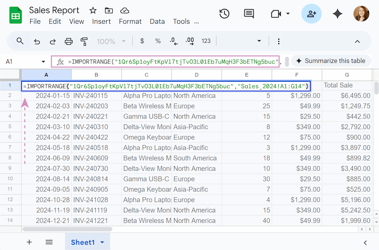
=IMPORTRANGE("1Qr6Sp1oyFtKpVl7tjTvO3L01Eb7uMqH3F3bETNg5buc","Sales_2024!A1:G14")
Let's look at each component in detail:
- =IMPORTRANGE: The start of the function.
- "1Qr6Sp1oyFtKpVl7tjTvO3L01Eb7uMqH3F3bETNg5buc": The ID of the source spreadsheet in double quotes.
- ,: A comma to separate the URL/ID from the range.
- "Sales_2024!A1:G14": The range string (also in double quotes), which consists of three key pieces of information:
- Sales_2024 is the name of the specific tab containing the data.
- ! is a separator between sheet name and range.
- A1:G14 is the exact range of cells we want to import.
- Press Enter.
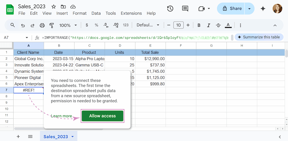
- On your first connection to a spreadsheet, the formula will return a #REF! error. Don't panic, that is as it should be: it's just IMPORTRANGE asking for access. Hover over the cell, and click the Allow access button.

- After granting access, your data will show up automatically.
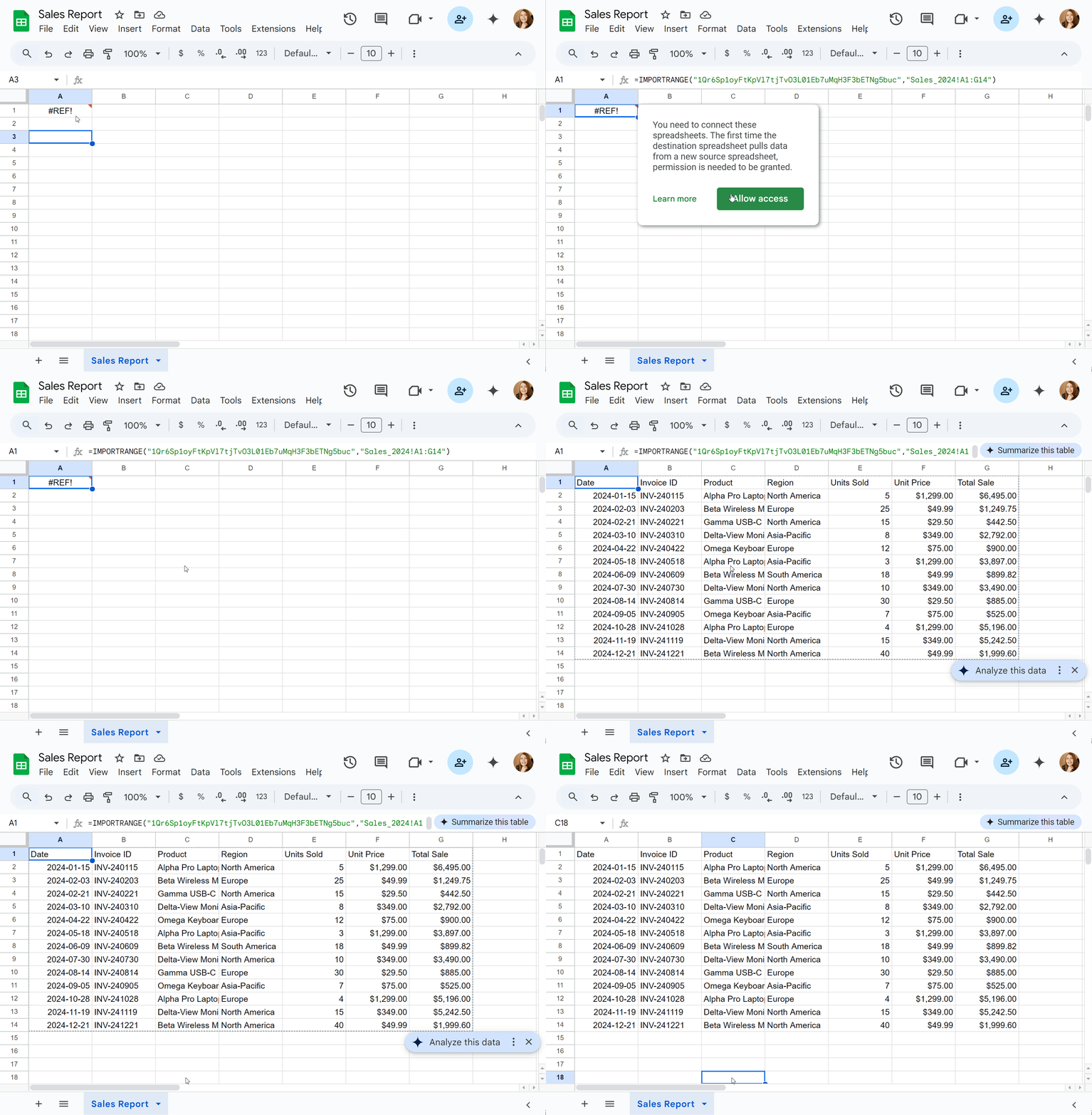
Note: Make sure you use standard straight quotes (") not curved ones (”). Spreadsheet formulas can only understand straight quotes.
Example 2. How to import multiple ranges in Google Sheets
We’ve figured out how to import the range from one sheet to another, but what if we need to import multiple ranges? Merging data from several sources by hand is quite difficult and it’s easy to mess up everything if there is a lot of data.
You could use two separate IMPORTRANGE formulas, but doing so often leads to a #REF! error because the formulas might clash and try to overwrite each other. Luckily, the array formula solves this by automatically adjusting the size of your data 😉.
IMPORTRANGE with array formula: vertical stacking into a single array
One of the most popular ways to combine datasets is to create a single array using curly braces {}. The curly braces in Google Sheets formulas combine data from multiple sources into one unified virtual table.
Note: This method works only when all your imported ranges have the exact same number of columns.
The IMPORTRANGE syntax for a combined array will look like this:
Let's look at some specific examples of how this function works.
Scenario A: IMPORTRANGE multiple tabs from the same spreadsheet
Your data may be located in one Google Sheet but spread across different tabs. Since the source is the same file, you need to use the same URL or ID for each part of the formula, changing only the sheet name (tab name) in the range string.
For example, you have sales data from the 2023 and 2024 years in two separate tabs within one spreadsheet. You need to combine them into one sheet, so you don't have to flip back and forth analyzing sales.
To import data from multiple tabs in the same spreadsheet, you’ll need the formula:
={IMPORTRANGE("1bajFlSE56gcgtaNQojQisG3vEL5e367_uGN1aIZfv30", "Sales_2023!A1:E6"); IMPORTRANGE("1bajFlSE56gcgtaNQojQisG3vEL5e367_uGN1aIZfv30", "Sales_2024!A2:E6")}
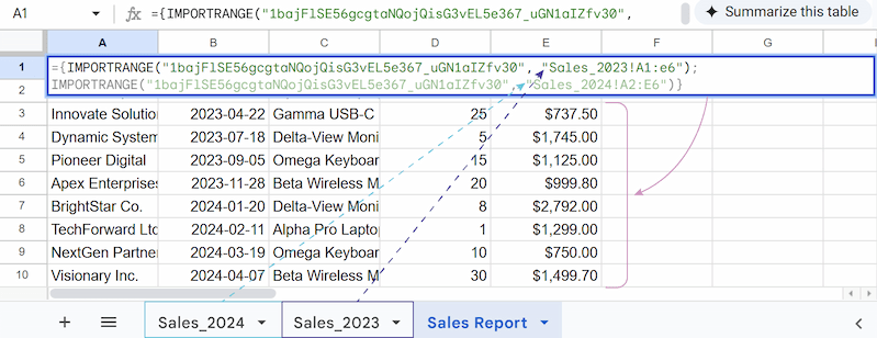
As you can see, we use the same ID for both IMPORTRANGE functions. The curly braces group them together, while the semicolon stacks the data vertically.
Tip: The second range we start from A2 instead of A1 to skip the header row of the second table so it doesn't appear in the middle of your combined list.
Scenario B: IMPORTRANGE from multiple sheets in different spreadsheets
Let’s take another example. Now you have sales data in two separate spreadsheets: one for 2023 and one for 2024. The array method still works for this case, but with a key difference - for each IMPORTRANGE we use a different URL/ID, as they are different documents.
Just add your specific file links and ranges like this:
={IMPORTRANGE("12_xJqvZXOrFa3p_6IBvBJ1Xa1DoMePvR6EHXHYkX9i","Sales_2023!A1:E6");IMPORTRANGE("15CJiyzbw-E9YpgLOEbWUWPttBJmrnI8lVIQHxz1WSv","Sales_2024!A2:E6")}
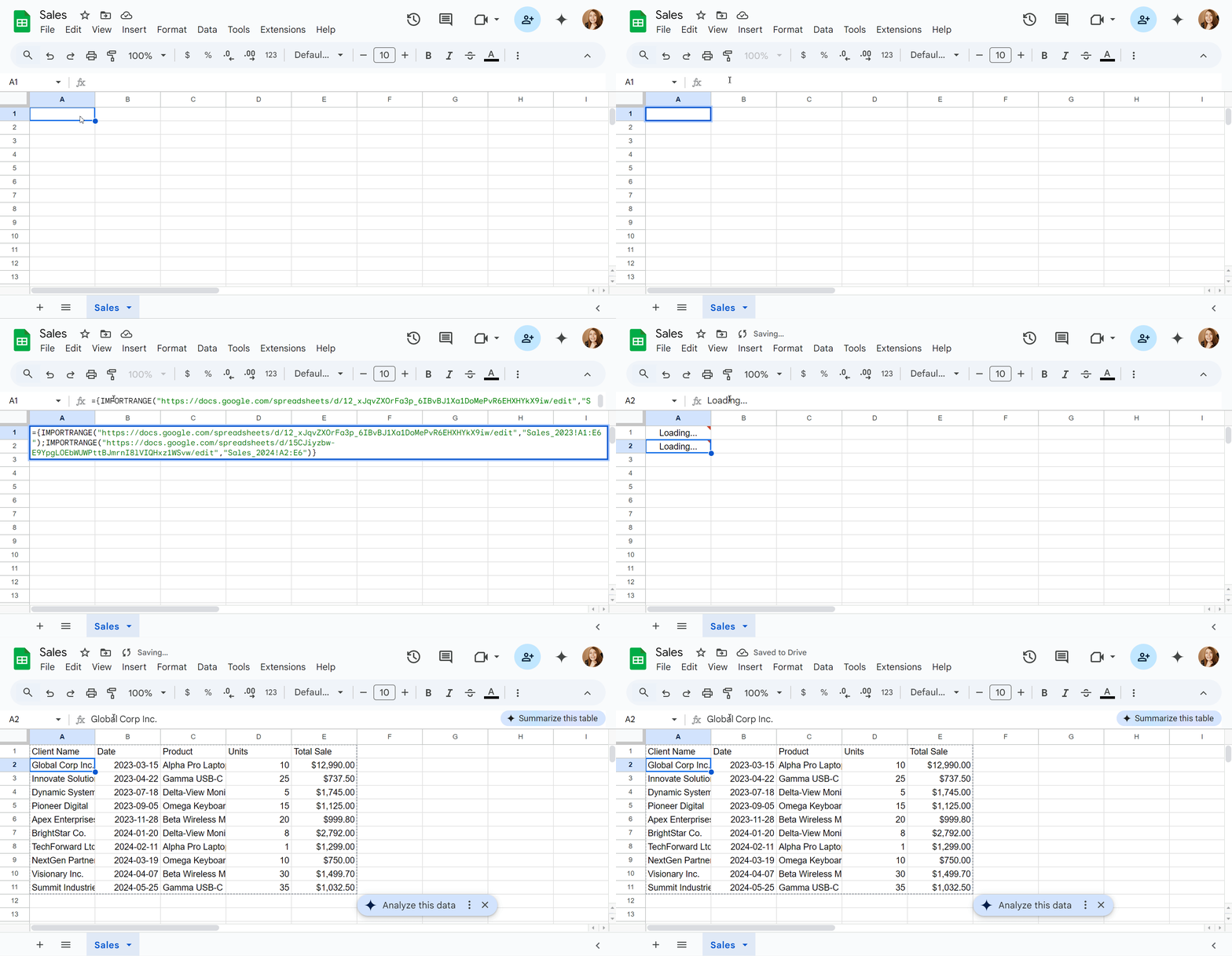
Let's take a closer look:
- ={...} are the curly braces that act like a container.
- IMPORTRANGE("12_xJqvZXOrFa3p_6IBvBJ1Xa1DoMePvR6EHXHYkX9i","Sales_2023!A1:E6") connects to your first spreadsheet and imports the sales data from the "Sales_2023" sheet in the range of "A1:E6".
- ; is a vertical stacking operator, which tells Google Sheets to place the next dataset underneath.
- IMPORTRANGE("15CJiyzbw-E9YpgLOEbWUWPttBJmrnI8lVIQHxz1WSv","Sales_2024!A2:E6") is the second function that imports the data from the "Sales_2024" sheet in the range of "A2:E6".
Note:
- #REF! Error: Unlike Scenario A, here you are connecting to different files. In this case, the Allow Access button often won't appear. If you see a #REF! error, try pasting each IMPORTRANGE part into a separate empty cell first. Click Allow Access for each one individually, and then combine them back into your array formula.
- #VALUE! Error: All ranges inside {} must have the exact same number of columns. If one range is A:E (5 columns) and another is A:D (4 columns), the formula will return a #VALUE! error.
All your imported data will combine into one master sheet.
Importing data with Combine Sheets
Formulas driving you nuts? The Ablebits suite of tools for Google Sheets is designed to replace them with easy-to-use applications. The add-ons act as an intuitive interface that builds complex formulas for you.
Combine Sheets is the perfect alternative to manually writing array formulas. The add-on itself generates a single, clean formula on your behalf.
It's easy to use, just follow these steps:
- Select the sheets you want to combine. You can pick them straight from your Google Drive.

- Choose the columns to combine.
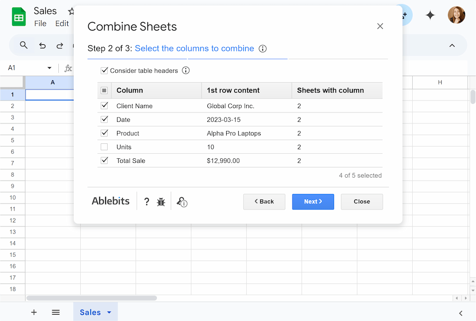
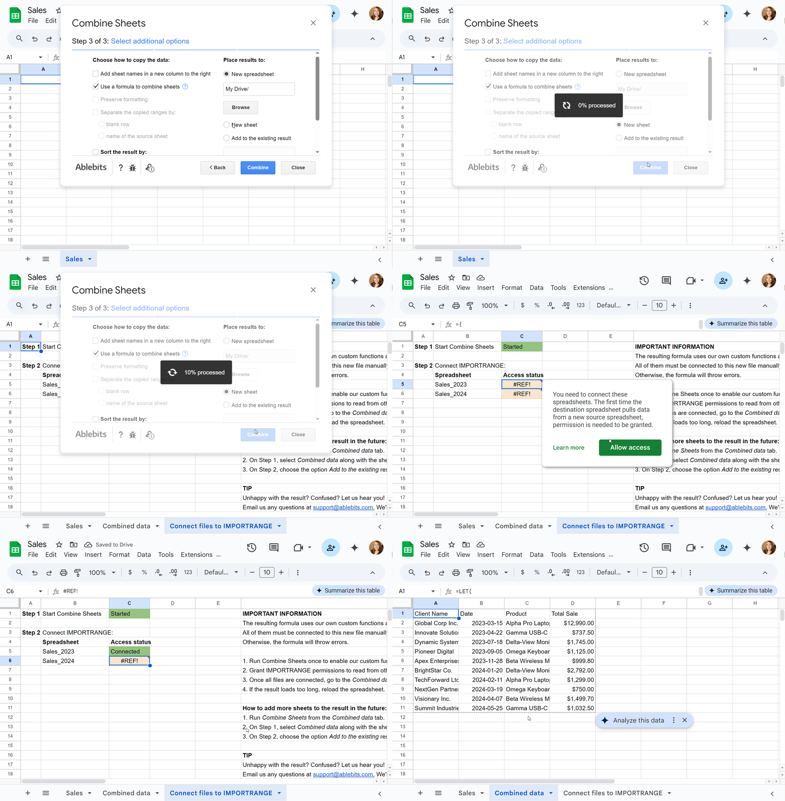
- Specify how to copy the data. Check the Use a formula to combine sheets box, and the tool will automatically generate the formula for you, keeping your data synced with the source.

- Pick where to paste results. After that, you’ll need to click Allow access buttons for the merging sheets, as the add-on uses an IMPORTRANGE formula inside. With just a few clicks, you’ll get perfectly merged sheets!
Example 3. How to import filtered range Google Sheets
The standard filter feature in Google Sheets modifies the view for everyone using the sheet. But what if you need to create a personal, live, filtered view of that master sheet without disrupting anyone else's work?
How to use the Google Sheets IMPORTRANGE FILTER combination
Instead of filtering the original sheet, you can pull the data into a new sheet using a powerful combination of the IMPORTRANGE and FILTER functions.
You'll need this formula pattern:
So, consider this scenario: a marketing manager needs a list of the team members and their start dates from the HR department to plan for anniversaries, but he must not see sensitive data like salaries from the Salary column. What should an HR manager do?
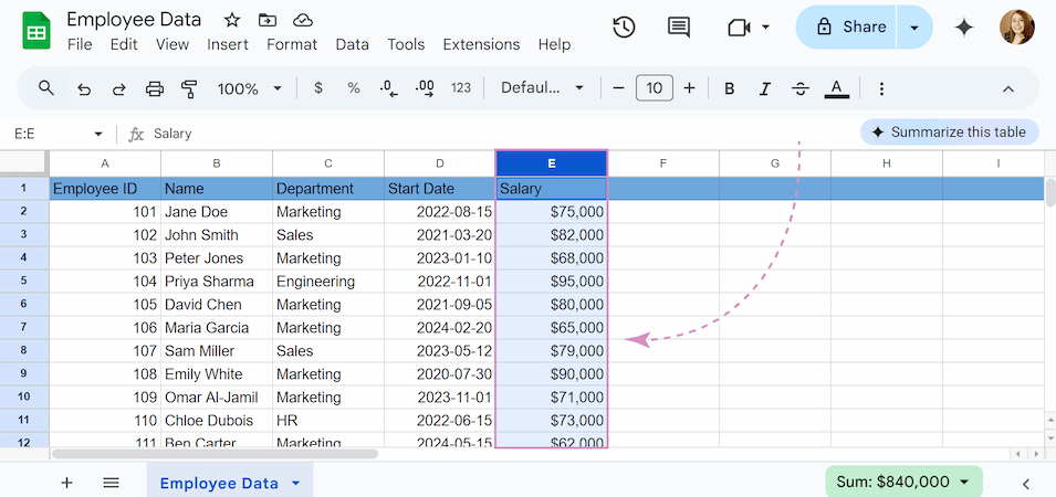
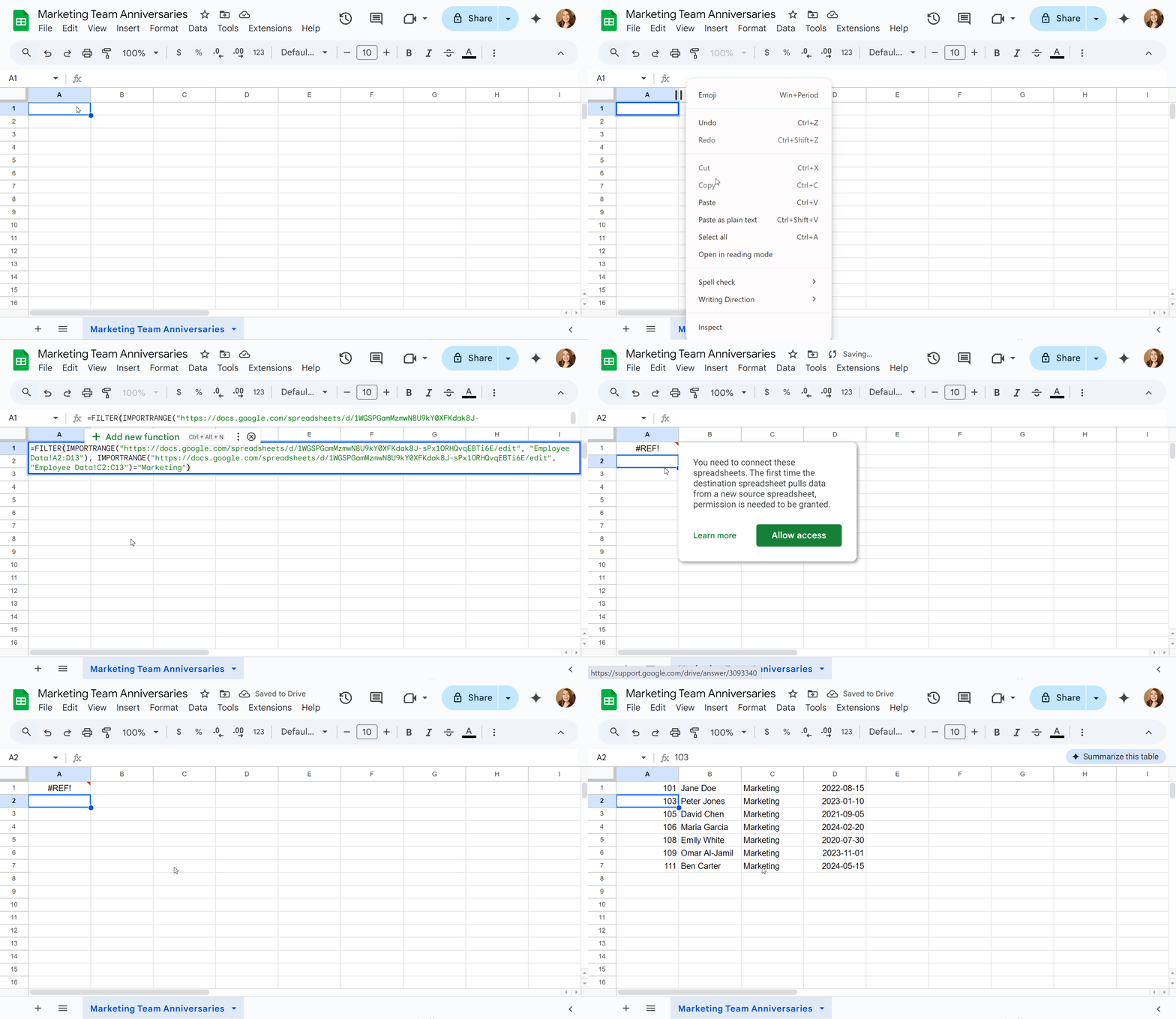
He can create a new, separate Google Sheet for the marketing manager. In A1, he uses a formula to import the data while carefully omitting the salary column:
=FILTER(IMPORTRANGE("https://docs.google.com/spreadsheets/d/1WGSPGamMzmwN8U9kY0XFKdak8J-sPx1ORHQvqEBTi6E/edit", "Employee Data!A2:D13"), IMPORTRANGE("https://docs.google.com/spreadsheets/d/1WGSPGamMzmwN8U9kY0XFKdak8J-sPx1ORHQvqEBTi6E/edit", "Employee Data!C2:C13")="Marketing")
Let's break down this formula:
- =FILTER starts our filtering function, which will display only rows that meet our criteria.
- IMPORTRANGE("https://docs.google.com/spreadsheets/d/1WGSPGamMzmwN8U9kY0XFKdak8J-sPx1ORHQvqEBTi6E/edit", "Employee Data!A2:D13") pulls the range A2:D13 from the "Employee Data" sheet.
- IMPORTRANGE("https://docs.google.com/spreadsheets/d/1WGSPGamMzmwN8U9kY0XFKdak8J-sPx1ORHQvqEBTi6E/edit", "Employee Data!C2:C13")="Marketing" checks C2:C13 and only keeps rows where the department equals "Marketing".
This formula displays only the rows where the department is "Marketing" and only shows the columns A through D. The Marketing manager now has a live, auto-updating list of his team members without information about their salaries.
Filter Google Sheets using the Filter and Extract Data add-on
While the FILTER function is powerful, it can quickly become overwhelming. Luckily, we have an ultimate solution: the Filter and Extract Data add-on.
Filter and Extract Data is filters values by multiple criteria and extracts ALL matching data. The best part? No formulas required.
Just see how easily we can complete the example:
- Select the table you want to filter.
- Choose which columns to include in your results. For our example, just uncheck the Salary box.

- Set the conditions. To do so, just select the option from the dropdown instead of typing it into a formula.

- Choose a place for the result.
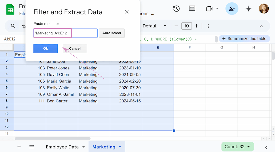
- Click Insert formula or Paste result.
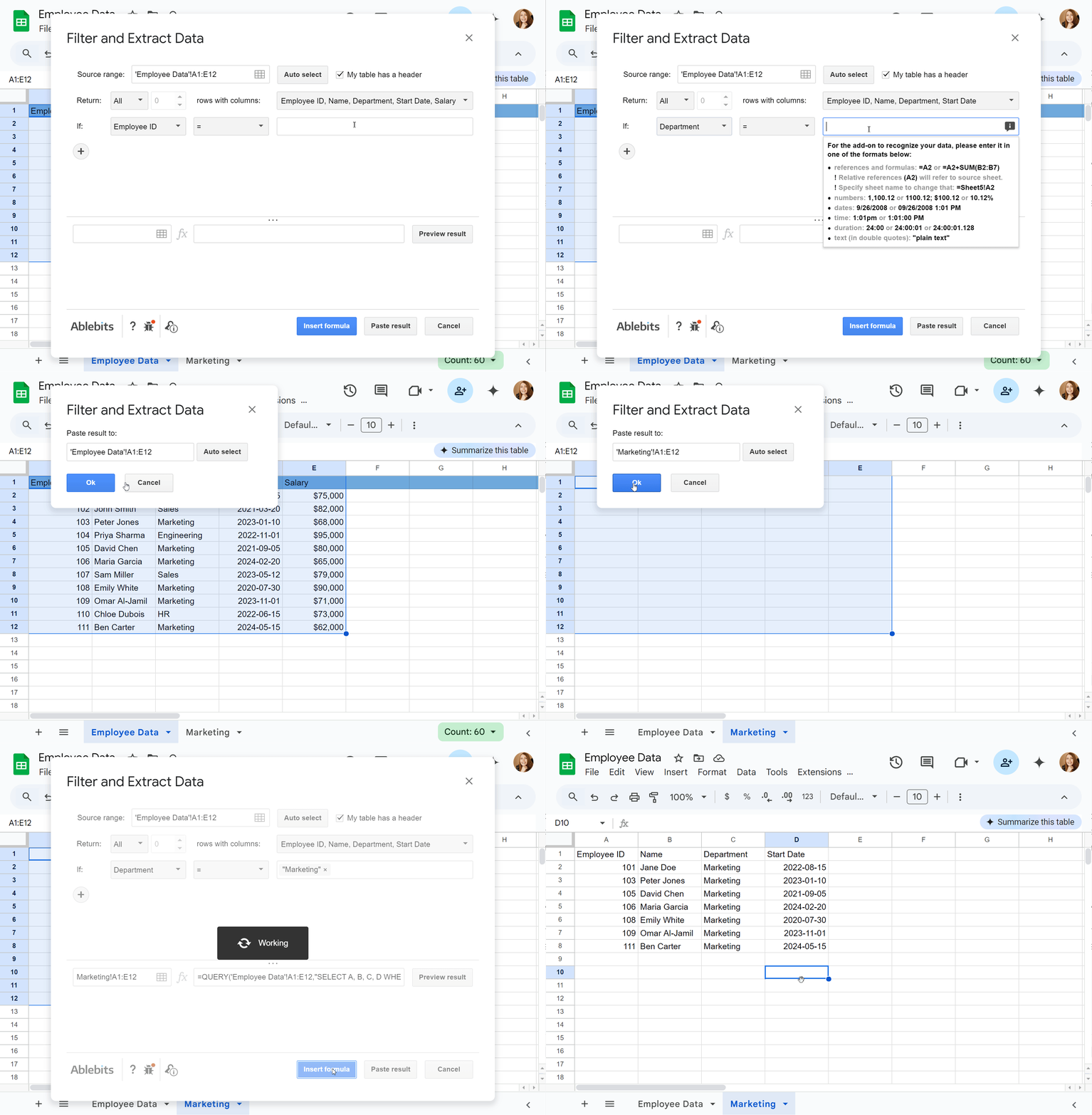
I highly recommend trying the Filter and Extract Data add-on for Google Sheets. It can significantly simplify how you work with your data, as it allows you to build complex filters through a simple visual menu, completely removing the need to write and debug complicated formulas.
Example 4. How to import specific columns in Google Sheets: QUERY IMPORTRANGE
IMPORTRANGE pulls a solid block of data, like A1:E10, by default. However, what if you only need several columns without the rest?
You can combine IMPORTRANGE with the QUERY function.
Tip: We have a comprehensive guide on the QUERY function in Google Sheets. Check it out for more detailed information.
The syntax of the QUERY IMPORTRANGE formula looks like this:
Note: You cannot use letters to refer to the columns. You must use Col + the number of the column relative to your range.
Let's take our table with sales data from 2024. For this example we just need to know the total sales of each product for the year and we don’t need any information about customers or purchases.
To import multiple columns in Google Sheets, we will use the formula:
=QUERY(IMPORTRANGE("1bajFlSE56gcgtaNQojQisG3vEL5e367_uGN1aIZfv30", "Sales_2024!C1:E6"), "SELECT Col1, Col3")
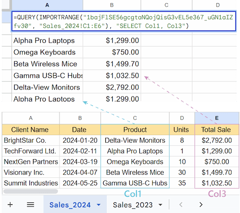
Let’s analyze how it works:
- QUERY takes the entire data provided by IMPORTRANGE and acts as a filter.
- SELECT Col1, Col3 is the rule that tells QUERY to return only the first and the fifth columns from the range.
Note: "Col1" refers to the first column of the range you imported, not the entire range of the table. So if your IMPORTRANGE starts at column C, Col1 would be column C, not column A.
As a result, you get a table with just the names and prices, dynamically linked to the source.
Example 5. How to use QUERY and IMPORTRANGE with conditions
Now we'll take a step further. Let's consider you have a large dataset in another spreadsheet and you only want to pull in the rows that meet certain conditions.
To do this, we'll add the WHERE clause to the QUERY IMPORTRANGE formula:
Imagine you have a main sheet "Finance" where daily or weekly financial transactions are logged. You want to import into a new spreadsheet only those rows where the "Status" column (Column 6) says "Paid".
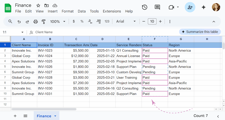
The perfect formula for this:
=QUERY(IMPORTRANGE("https://docs.google.com/spreadsheets/d/19mA0-2Cph5BJ38NjgVeTmA3Wdbnhj2aacSol9nBJsHs/edit","Finance!A2:G10"), "SELECT * WHERE Col6 = 'Paid'")
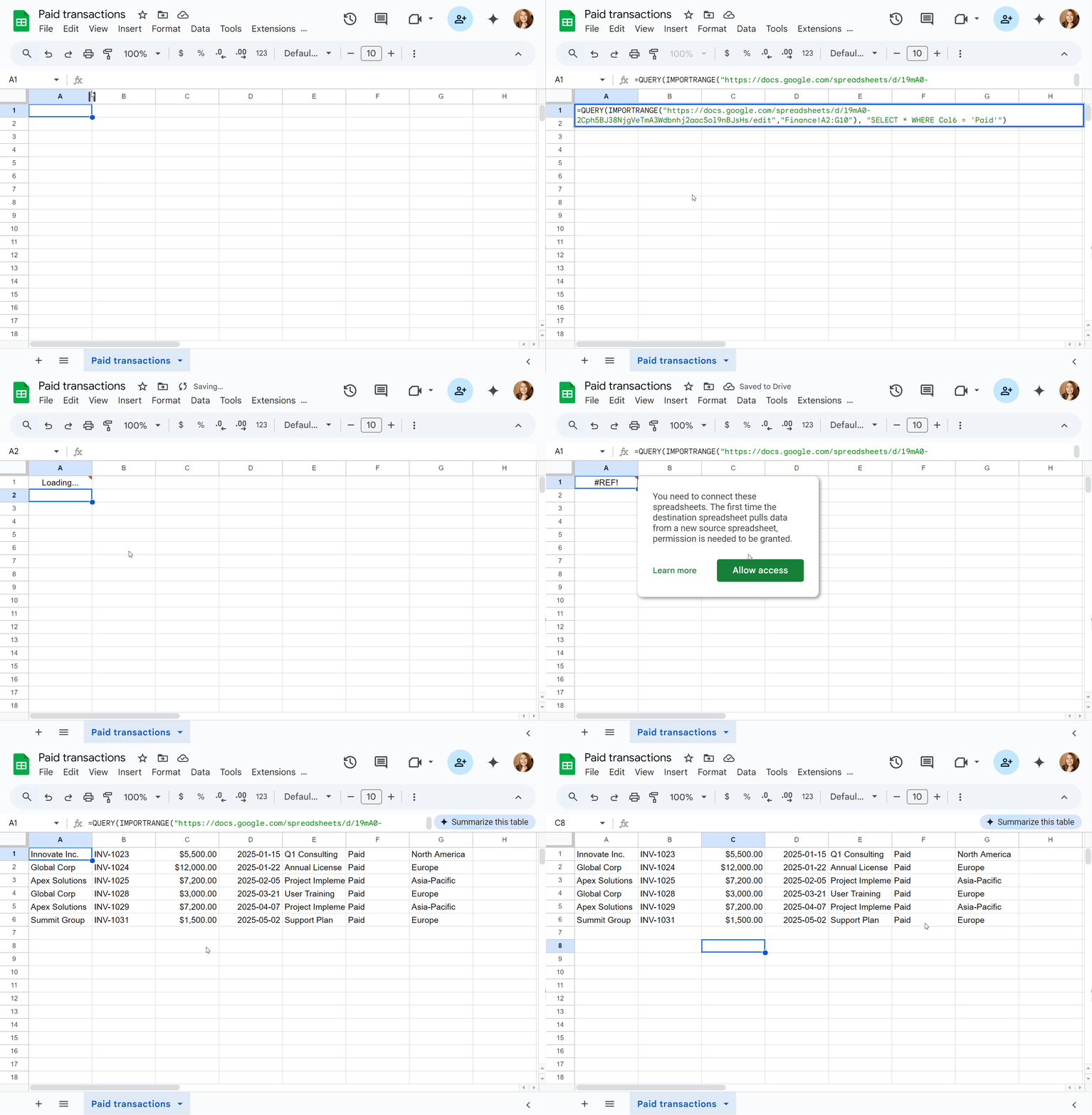
A step-by-step explanation is as follows:
- QUERY(...) allows you to filter the data.
- IMPORTRANGE("https://docs.google.com/spreadsheets/d/19mA0-2Cph5BJ38NjgVeTmA3Wdbnhj2aacSol9nBJsHs/edit","Finance!A2:G10") connects to your source sheet "Finance" and grabs the data in the range from cell A2 to G10.
- SELECT * tells the function to return every column from the data that was imported.
- WHERE sets the condition for which rows to show.
- Col6 = 'Paid' is the condition itself. It instructs the formula to look at the 6th column of the imported data and only show the rows where the value in that column is 'Paid'.
Note. When using QUERY with IMPORTRANGE, you must refer to columns by number (Col1, Col2, Col3), not by letter (A, B, C).
Now the most important thing is that when you add new transactions to your original file, the other spreadsheet with imported data will be updated automatically without your participation.
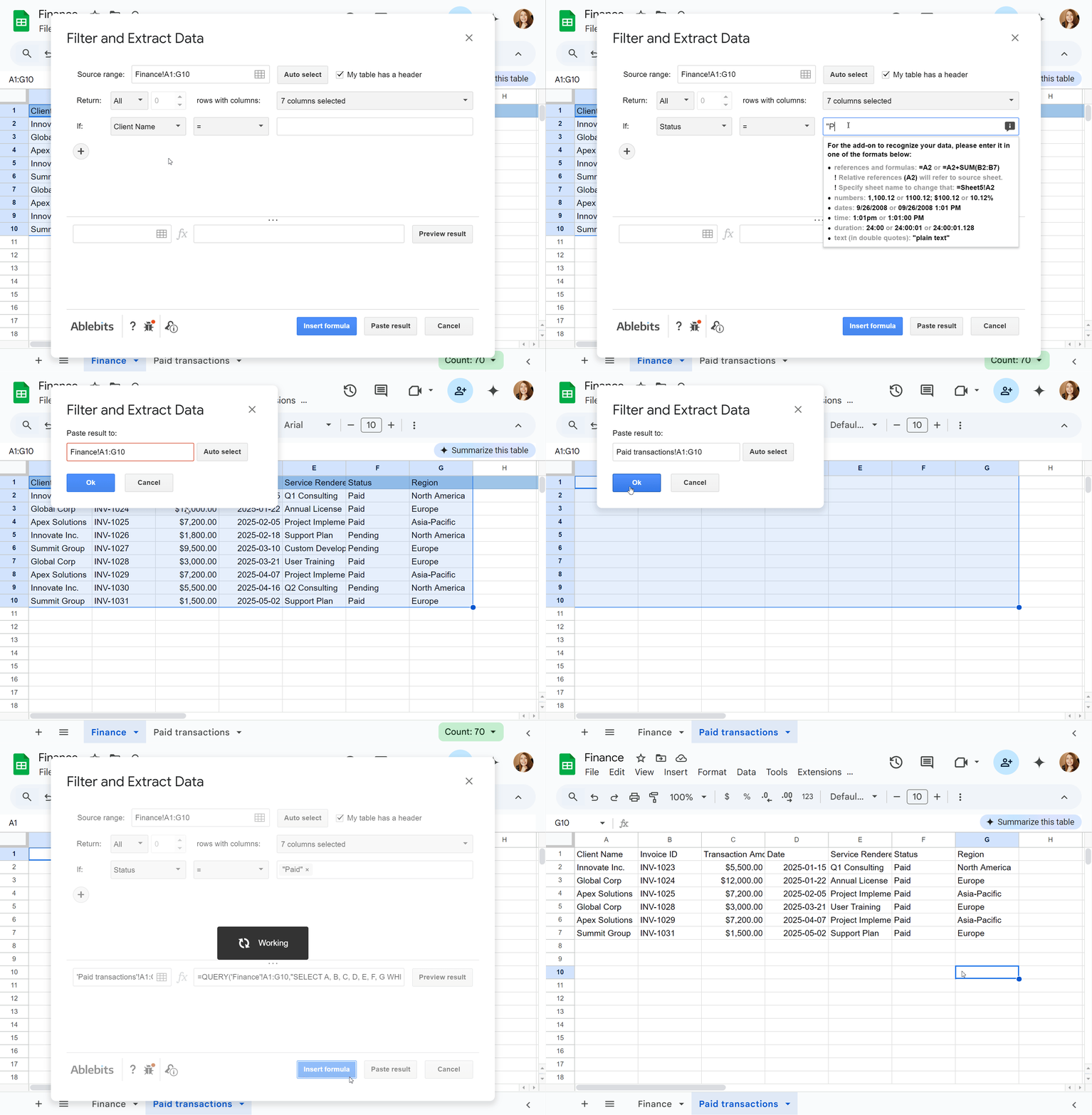
Stuck on the formula? The Filter and Extract Data add-on can easily bail you out here too! Just set up your condition with a few clicks and select a place for the result. The tool will pull the clean, filtered data into a new sheet for you, creating the same live, auto-updating list without the headache.
Example 6. How to VLOOKUP with IMPORTRANGE in Google Sheets
We've learned how to import blocks of data and even specific columns. But what if you don't need a whole list? Let's return to our "Finance" table. We have "Invoice IDs" here, and in this example we just want to find and import into another spreadsheet the "Payment Status" of the specific invoice.
In this case, you can use another Google Sheets formula combination: VLOOKUP + IMPORTRANGE.
Tip: Read more about the syntax of the Google Sheets VLOOKUP function and how to use VLOOKUP formulas in this article.
The VLOOKUP IMPORTRANGE formula looks like this:
=VLOOKUP("INV-1025", IMPORTRANGE("19mA0-2Cph5BJ38NjgVeTmA3Wdbnhj2aacSol9nBJsHs", "Finance!B2:F10"), 5, 0)
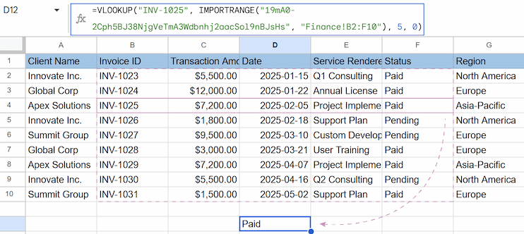
Let's look at the components:
- "INV-1025": It’s the specific invoice you are looking for (you can also reference a cell, like A2). In other words, it's your search key.
- IMPORTRANGE("19mA0-2Cph5BJ38NjgVeTmA3Wdbnhj2aacSol9nBJsHs", "Finance!B2:F10"): This is the part where we're telling the function in what range to search.
Note: We intentionally start the range from Column B (not A) because VLOOKUP always searches for the key in the first column of the selected range.
- 5: This is the Index. We want the value from the 5th column of our imported range (Counting from B: B=1, C=2, D=3, E=4, F=5). Column F contains the Payment Status.
- 0: This ensures an Exact Match.
Tip: If you see a #REF! error, the VLOOKUP wrapper might be hiding the Allow Access button. To fix this, paste just the IMPORTRANGE part into a separate empty cell first, click Allow Access, and then delete it.
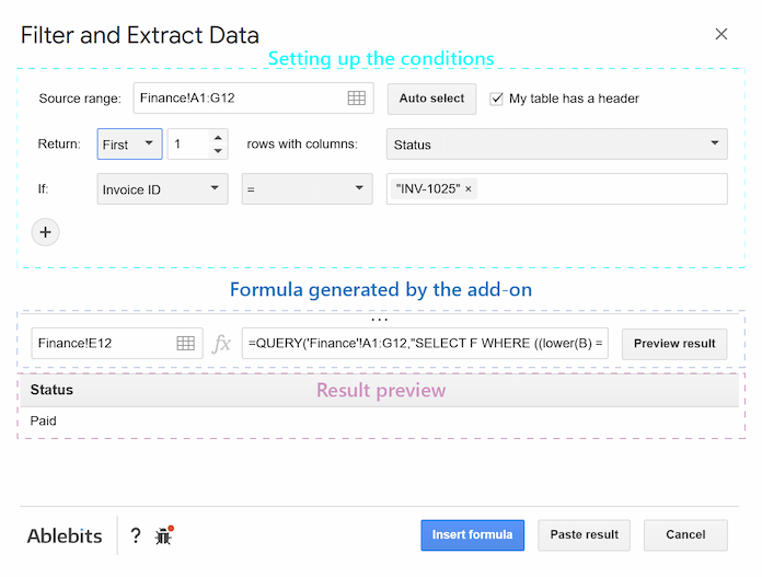
If this VLOOKUP formula looks a bit daunting, the Filter and Extract Data add-on can handle this task too. It automatically generates the correct formula for you, so you don't have to worry about mixing up ranges or column indexes.
That's how you can use the IMPORTRANGE function and add-ons to connect Google Sheets for live data updates. I hope you master IMPORTRANGE with all this information. Below, I'll cover the most common mistakes, in case you encounter any, and answer the most frequent questions 👉.
Google Sheets IMPORTRANGE function not working? Common errors and solutions
#REF! error
This is the error you'll see 90% of the time using the IMPORTRANGE function. It's a general error. This one may hint at several things:
- IMPORTRANGE doesn’t have access to the file yet. You are trying to grab data from a spreadsheet for the first time, and Google needs your permission to link.
Solution: Hover over the cell with the #REF!, an Allow access button will appear. Click this button.
- Incorrect URL or sheet/range name. The formula can't find the file or the specific tab/cells you told it to look for.
Solution: Go to the source spreadsheet and check its URL directly from your browser's address bar. You could have lost a couple of characters when you shortened the formula. Also double-check that the sheet name in the formula exactly matches the name of the tab in the source sheet and the range you've specified actually exists on that sheet.
- You don't have permission to the source sheet. It may occur that the Google account you are currently logged in with does not have at least "View" access to the source spreadsheet.
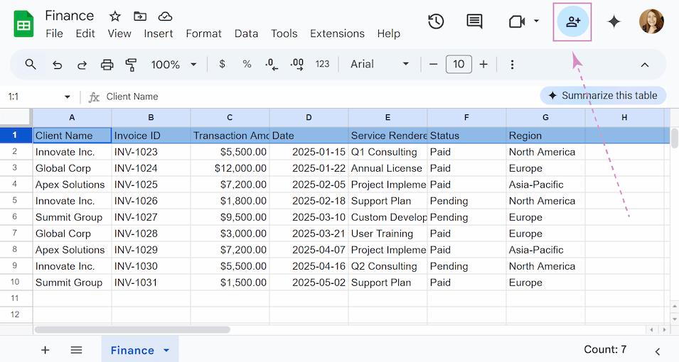
Solution: Go to the source spreadsheet you are trying to import from and click the Share button in the top-right corner. Ensure that your email address is listed with at least "Viewer" permissions. If it's not, ask the owner of that sheet to share it with you.
- Overwriting data. IMPORTRANGE needs enough empty cells below and to the right of it to display all the imported data. The error tells you that there is already something in one of those cells.
Solution: Look at the cell address mentioned in the error message. Go to that cell and delete its contents. The formula should then work correctly.

#ERROR! error
There is a syntax mistake in your formula. Google Sheets cannot understand the instructions you've written.
Solution: The most common cause is the missing quotation marks. Double-check both the spreadsheet_url and the range_string. They must be enclosed in double straight quotation marks ("). Also, make sure there is a comma separating the URL from the range string.
#VALUE! error
It often means the error isn't with the import itself, but with a function you've wrapped around it (like QUERY, FILTER, or other). But sometimes an access problem may show this error.
Solution: Separately copy each IMPORTRANGE(...) part of your formula and paste it into a new, empty cell. Does it work on its own? One of these cells will likely show a #REF! error. Hover over that cell, and a button will appear asking you to Allow access. You must grant permission for each unique spreadsheet you are linking to.

If it returns the data correctly, you know the problem is 100% in your outer function. Check the wrapper. For example, the QUERY function has very strict rules: a small syntax error may cause the whole formula to fail.
#N/A error
This error means that no data matches your filter conditions.
Solution: The first step is to confirm the data is arriving correctly. As with the #VALUE! error copy just the IMPORTRANGE(...) part of your formula and check if it returns #REF! error (the problem with access to the spreadsheet may exist here too). If it's a #REF!, use the solutions earlier in this article to fix the connection first.
If the import works, the problem is with your FILTER logic. Look closely at the condition you are filtering by. Is there a typo? Does any of the data actually meet the criteria you've set?
To make your filtered data more presentable when no results are found, wrap your formula with IFNA. In this case, the standard #N/A error will be replaced by a custom message. For example:
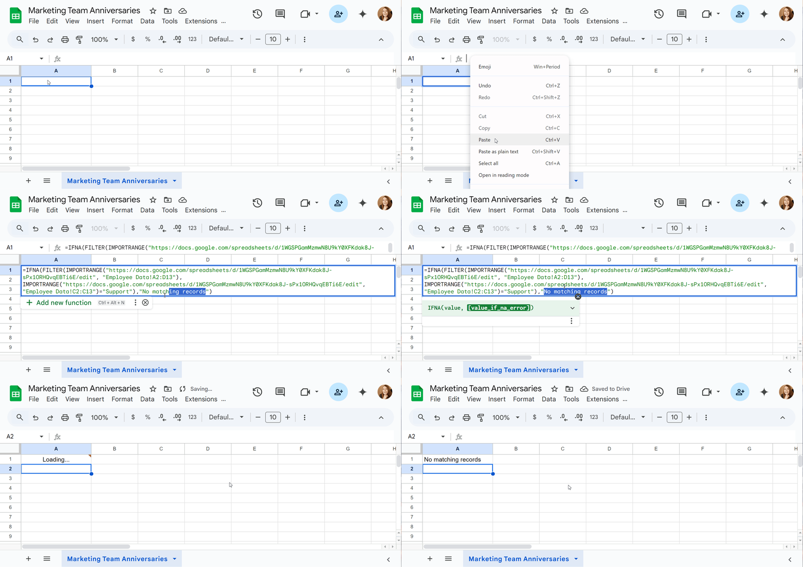
The formula works exactly as before when results exist, but now displays "No matching records" instead of an error when the filter comes up empty. You can replace this text with any message you prefer, or use empty quotes "" to leave cells blank.
"Loading..." issue
If the "Loading..." message hangs indefinitely or your spreadsheet responds very slowly, a formula may be stuck. The syntax and formula structure are correct, but the issue occurs due to data limits or an unexpected bug. This can make your whole spreadsheet slow or even freeze completely.
Google's official documentation warns that the "Loading..." issue can be caused by too many requests. You may see the message: "Error Loading data may take a while because of the large number of requests."
To resolve this, Google recommends reducing the number of import functions used across your spreadsheets.
The official documentation points out key official limits to be aware of:
- 10MB of received data per request.
- The 600-user share limit for the source sheet.
But the official documentation doesn’t cover the bulk of the difficulties when you encounter this error. Let’s have a look at the most frequent user-reported loading issues and their solutions:
- You hit a data wall. User experience suggests a limit of around 50,000 cells. In our tests, with text-heavy cells, this number drops to around 15,000 cells.
Solution: Import only what’s necessary (For example, specify ranges like A1:D100 rather than entire columns).
- Too many separate requests. Each IMPORTRANGE is quite a heavy request. Having too many individual formulas affects performance and can trigger usage limits and cause errors.
Solution: Use a single IMPORTRANGE formula to bring all the necessary data into a dedicated sheet, rather than making additional IMPORTRANGE calls in individual cells. Then, you can refer to that dedicated sheet as much as you need.
- Complex calculations. The receiving spreadsheet cannot display imported data until every calculation is completed in the source spreadsheet.
Solution: Filter/aggregate in the source sheet first and only then import the data (For example, sum rows there in the source sheet and import the total). For maximum control in complex workflows, especially if live feed is not necessary, consider using dedicated tools. Add-ons like Combine Sheets, Filter and Extract Data, or Split Sheet can import static data to the target spreadsheet, which eliminates refresh delays.
- Imports that depend on other imports. Your final sheet must wait for every other sheet in the chain to finish loading first.
Solution: Create a "Data_Hub" sheet with one IMPORTRANGE to pull all source data and reference this local copy for all calculations instead of repeating imports.
- Unpredictable bugs. Sometimes random "Loading..." freezes without clear triggers. 😓
Solution: Refresh your browser or wait several minutes for the spreadsheet to recover.
- Incorrect file format. If you are trying to import data from an Excel file (.XLSX) stored in Google Drive, it can cause persistent loading failures.
Solution: Convert to Google Sheets. Avoid .XLSX files and save as native Google Sheets format.
Frequently Asked Questions (FAQ)
What is the difference between IMPORTRANGE and simple copy-pasting?
When you are copy-pasting information, you create a static copy, like a screenshot, with no link back to the original file. Even if someone updates something later, your copy won't change. IMPORTRANGE, on the other hand, keeps a real-time connection with the source file. Any updates in the original sheet automatically appear in your sheet.
Does IMPORTRANGE have a data limit?
The IMPORTRANGE formula can only import data of 10 MB maximum. If the range you select is too large, you will get an error. Moreover, while Google's official documentation is not explicit on a hard limit, there's a practical cap on performance. Historically, a single sheet could reliably pull data from up to 50 different source spreadsheets. Going over this limit can slow down your sheet and cause errors. To overcome this, you can use a dedicated tool. For example, the Combine Sheets add-on is perfect for large-scale projects or reports.
How to import ranges from one sheet to another and preserve formatting?
IMPORTRANGE copies data only without any of the original formatting (like colors, fonts, or borders). You'll need to manually reformat the imported data to match your style. If keeping the original formatting is important to you, it would be useful to try out the Combine Sheets add-on. It merges data while perfectly preserving all the source formatting, saving you time and hassle.
Why do I keep getting the #REF! error?
This is almost always a one-time permission issue. For security, Google Sheets requires you to grant access for one sheet to pull data from another. You only have to do this once for each unique spreadsheet you connect to.
Is there any difference between IMPORTRANGE and IMPORTDATA?
Yes. IMPORTRANGE imports data from another Google Sheet into your current sheet. IMPORTDATA brings in data from public web files like CSV or TSV formats. They're both for importing, but work with completely different sources: IMPORTRANGE for spreadsheets, IMPORTDATA for web data files. The big differences? IMPORTRANGE needs sheet access and updates every 30 minutes, while IMPORTDATA works with public links but refreshes only hourly.
My formula is making my sheet slow. What can make it work quicker?
If your sheet is slow due to IMPORTRANGE, try importing only what’s necessary. This will reduce data load. For complex tasks like merging or filtering large datasets, use optimized tools like our Filter and Extract Data or Merge Sheets add-ons instead of manual formulas — they’re designed for speed!
Is there a formula-free way to combine data?
Absolutely. While you can manually stack data with array formulas like ={IMPORTRANGE(...); IMPORTRANGE(...);...}, this can be tricky to debug. This is a perfect scenario for using a dedicated tool. For a much simpler, no-formula solution, add-ons like Combine Sheets or Merge Sheets are designed to merge multiple sheets in a few clicks, saving you time and preventing errors.
How to split Google Sheets?
You may create new Google Sheets for each split category. Then, use IMPORTRANGE in each new sheet to import only the matching rows. But it’s time-consuming if you have many splits. The best way is to use special add-ons like Split Sheet. It generates the correct formula in each new sheet it creates, giving you a complete set of live, auto-updating sheets in seconds.
How to archive data in Google Sheets?
This is a simple but crucial two-step process. First, you pull the live data using IMPORTRANGE. Second, you must break this link: select all the imported cells, copy them, and then Paste as values only. The formula will be replaced by the static data, creating an archive.
Hope this guide makes IMPORTRANGE easier to use! If anything’s still unclear or you’ve got a tricky use case — drop your question in the comments below. Your questions could shape the next post 😉
 by
by