This tutorial explains how to use regex match in the XLOOKUP and XMATCH functions to check patterns, validate formats, and run more flexible lookups.
Excel XLOOKUP and XMATCH are strong functions on their own, and regex match makes them even more versatile. Instead of searching for exact text, you can now use full-blown regular expressions to define what you are after.
In this tutorial, you will learn:
What is regex match in XLOOKUP and XMATCH?
When you need to retrieve information based on patterns rather than exact values, the classic match mode options in XLOOKUP and XMATCH can feel limiting. Regular expressions change that.
With the regex match mode, the functions can look up values that match a specific pattern such as:
- ID, SKU, invoice number, or product code
- Email addresses and web links
- Strings that start or end in a certain way
- Text that contains this OR that
How XLOOKUP and XMATCH with regex work
To enable regex matching in the XLOOKUP and XMATCH functions, you basically need two things:
- Set the match_mode argument to 3.
- Include a regex pattern in lookup_value.
Here is the generic XLOOKUP formula with regex match:
And this is the XMATCH function with regex:
Conceptually, the functions with regex match mode work in this way:
- Take the regex pattern from lookup_value.
- For each cell in lookup_array, check whether it matches that pattern using Excel's regex engine.
- Return the match:
- XLOOKUP returns the first value from return_array where the pattern matches.
- XMATCH returns the relative position of the first value in the lookup_array that matches the regex pattern.
Key points:
- The regex can match any part of the cell value, unless you anchor it with ^ (start) or/and $ (end).
- The lookup value is not a "literal text" – it is an expression that describes what you want to match.
- You can still use the optional if_not_found and search_mode arguments as usual.
Tip. If you do not feel comfortable with regular expressions yet, you can start with our Excel Regex cheat sheet for beginners.
In what Excel versions is regex match available?
At the time of writing, regex matching in XLOOKUP and XMATCH is only supported in Microsoft Excel 365 for Windows and Mac.
If you don't see this feature in your Excel, you may need to update your Microsoft 365 to the latest version.
How to use Excel XLOOKUP with regex match
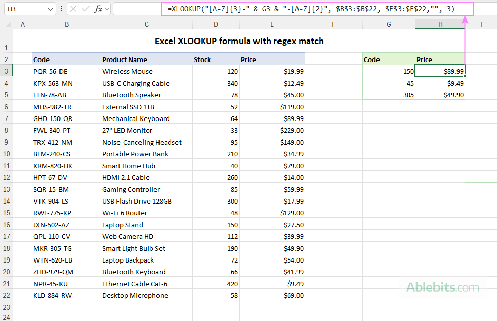
To see how regex match works in a real example, imagine a simple inventory list where column B contains product codes in range B3:B22. Each code has three groups of characters separated by hyphens (for example, ABC-12-DE or ABC-123-DE).
You want to look up the item price based on just the middle number entered in a certain cell (G3).
To fulfill the task, you first build the regex pattern for your code format:
[A-Z]{3}-\d{2,3}-[A-Z]{2}
Where:
- [A-Z]{3} – three uppercase letters
- \d{2,3} – two or three digits
- [A-Z]{2} – two uppercase letters
- - is a literal hyphen
Because we are searching for the numeric part typed in G3, we turn this static regex pattern into a dynamic one by concatenating the cell reference into the middle: "[A-Z]{3}-" & G3 & "-[A-Z]{2}"
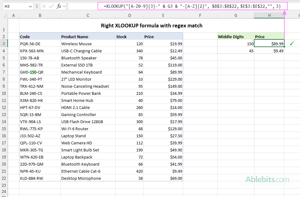
Assuming, the codes are in B3:B22 (lookup array), prices are in E3:E22 (return array), and the number to search for is in G3 (lookup value), enter this formula in H3:
=XLOOKUP("[A-Z]{3}-" & G3 & "-[A-Z]{2}", $B$3:$B$22, $E$3:$E$22,"", 3)
As a result, Excel finds the first code where the middle part matches the number in G3 and returns the corresponding price from column E.
What the formula does:
- Interprets the lookup value as a regex because match_mode = 3
- Searches column B for the first code that matches your regex pattern.
- Returns the corresponding value from column E in the same row.
Please note that we use the dollar sign to fix the lookup and return ranges, so you can copy the formula down to match the value in G4 and G5 without the ranges shifting.
How to use Excel XMATCH with regex
Sometimes you don't need to return a value and simply want to know where something appears in a list. This is where XMATCH comes in handy. And with regex support, it can handle a wide range of pattern-based searches.
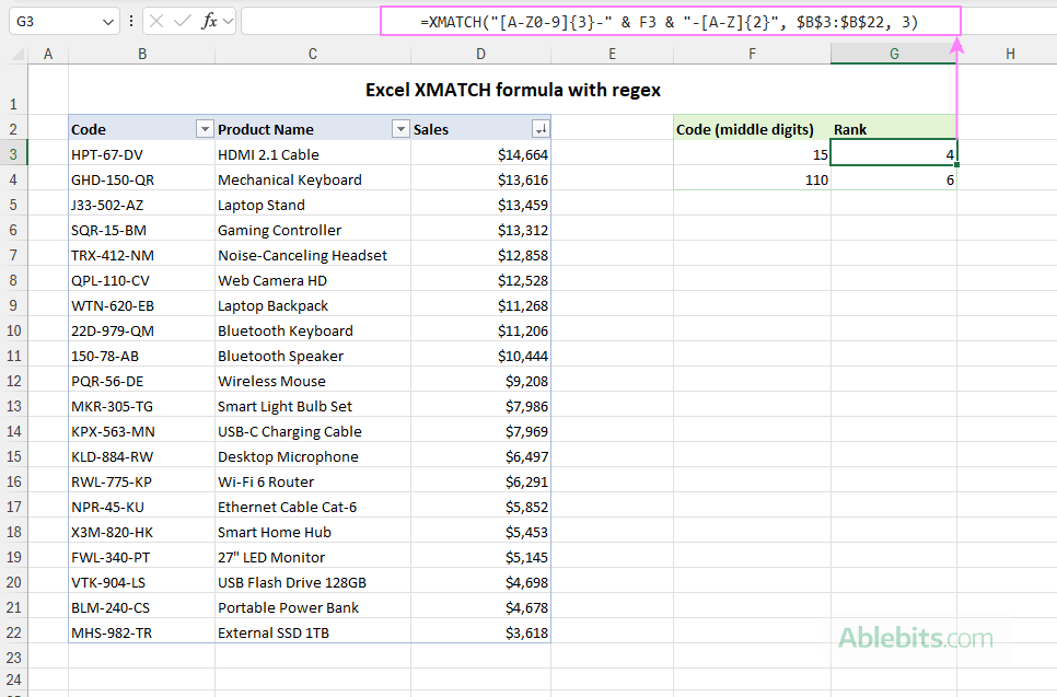
Suppose you have a worksheet where:
- Column B contains product codes such as SQR-15-BM or QPL-110-CV.
- Column C contains sales amounts, sorted from highest to lowest.
- Cell F3 holds the middle digits of the code of interest (for example, 15 or 110).
Your goal is to find out where that product stands among all sales. In other words, you want to know the ranking position in the sorted list.
Because the middle digits vary, and the rest of the code follows a fixed structure, you can create a dynamic regex like we already used in the XLOOKUP example above:
=XMATCH("[A-Z0-9]{3}-" & F3 & "-[A-Z]{2}", $B$3:$B$22, 3)
Enter this formula in the cell where you want the ranking result (G3 in this example). If you plan to look up several codes, just copy it down.
What the formula does:
- Treats the lookup value as a regex because match_mode = 3
- Searches column B for the first code that matches your regex pattern.
- Returns its position within range B3:B22.
Since column C is sorted in descending order, the XMATCH output directly shows where that product falls within the sales list. For example, a result of 1 means it's the top-selling item, a result of 2 means it ranks second among all products, and so on.
Why use full regex patterns in Excel functions?
Because regular expressions can match any part of a cell's content, you may be tempted to search for just the part of the lookup value you're interested in. In small or neatly structured datasets this can appear to work, especially when that fragment is unique.
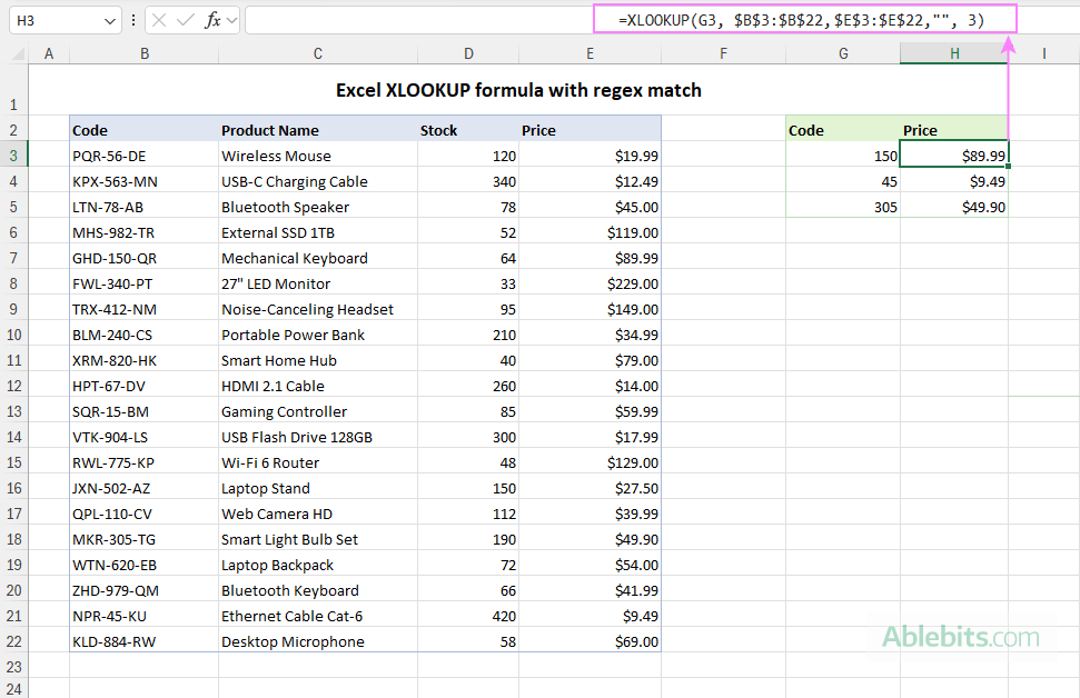
Although this method is very simple (and even recommended in some online tutorials), it is not accurate and can easily lead to incorrect matches.
For example, if the first part of your codes can contain both letters and digits, the below formula will stop searching as soon as it finds the specified number in any position within the code:
=XLOOKUP(G3, $B$3:$B$22, $E$3:$E$22, "", 3)
This tells Excel:
Find the first code that contains this number anywhere.
… which is not the same as:
Find the code where this number appears in the middle group.
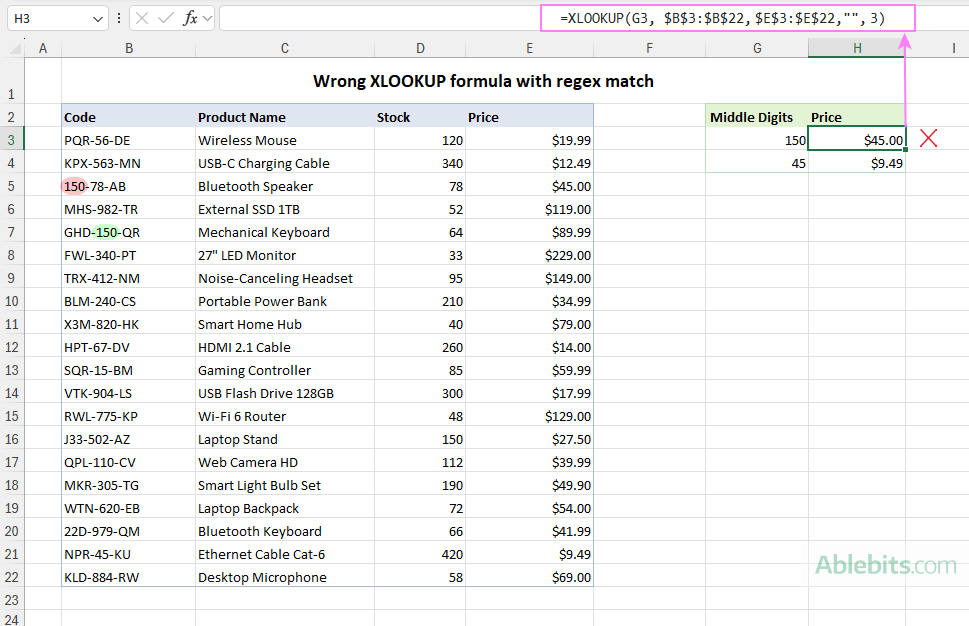
To avoid false matches, you need to define the entire structure of your lookup value in the regex pattern. In our case, it is:
"[A-Z0-9]{3}-" & G3 & "-[A-Z]{2}"
Here:
- [A-Z0-9]{3} matches three alphanumeric characters (any uppercase letter or any digit).
- [A-Z]{2} matches the final two uppercase letters
- - matches the literal hyphens
With the complete regex pattern in place, the XLOOKUP formula takes this form:
=XLOOKUP("[A-Z0-9]{3}-" & G3 & "-[A-Z]{2}", $B$3:$B$22,$E$3:$E$22,"", 3)
This tells Excel to return the price for the item whose middle digits match the value you entered in G3, and only for codes that follow the specified format.
Formula examples of regex-based XLOOKUP and XMATCH
To understand how useful regex match can be, let's walk through a few more practical examples.
Example 1. Lookup values that start with or end with certain text
Let's say you have a dataset where column B contains customer IDs and column C lists customer names. Each ID uses a short code format, such as EU-001, US-123, or 450-US. Notice that the country code may appear either at the beginning or at the end of the ID.
You aim to pull the customer name for an ID that starts with a certain country code or ends with one. Here's how to build both formulas using regex match in XLOOKUP.
Formula A. Lookup strings that start with specific letters
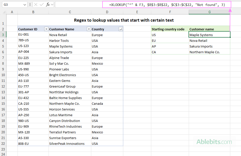
Let's assume cells F3 to F6 contain the starting patterns you want to match, such as "US" or "EU".
To retrieve the customer name from column C, use the regex start anchor ^:
=XLOOKUP("^" & F3, $B$3:$B$22, $C$3:$C$22, "Not found", 3)
This looks for IDs that begin with the text typed in F3. Copy the formula down to check prefixes in cells F4:F6.
Formula B. Lookup strings that end with specific letters
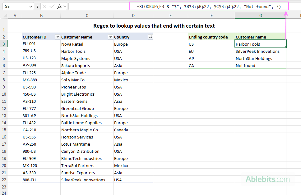
Now, let's match ending patterns entered in the same cells (F3:F6).
To find IDs that end with those letters, use the regex end anchor $:
=XLOOKUP(F# & "$", $B$3:$B$22, $C$3:$C$22, "Not found", 3)
This returns the first ID that ends with the letters in F3. To get matches for country codes in F4:F6, drag the formula down as needed:
Formula C. Using full regex pattern
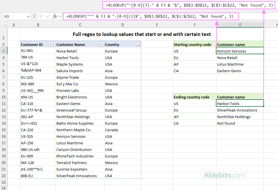
If column B contains mixed formats (different separators, unpredictable characters, or inconsistent lengths) you may need a more complete pattern to ensure the match happens in the correct place.
For IDs that start with a country code followed by a hyphen and three digits:
=XLOOKUP("^" & F3 & "-[0-9]{3}$", $B$3:$B$22, $C$3:$C$22, "", 3)
For IDs that end with a country code preceded by three digits and a hyphen:
=XLOOKUP("^[0-9]{3}-" & F3 & "$", $B$3:$B$22, $C$3:$C$22, "", 3)
Using the full pattern prevents false matches and makes sure the lookup aligns with the ID structure you expect.
Example 2. Regex to look up and match one of several options (OR pattern)
For this example, consider a table where column B lists team names and columns C and D store wins and losses, respectively. Each team name includes a state, sometimes written in full, sometimes as a two-letter abbreviation. For instance, you might have Dragons CA or Storm New York. Each state appears only once in the list.
Your goal is:
- To get the number of wins and losses for a specified state, taking into account that it may appear as either an abbreviation or a full name.
- After that, to sort the table by wins and find the ranking of the team from that state.
This is a perfect case for the alternation (OR) regex construct that matches one of several options.
Formula A. XLOOKUP with OR regex
Suppose you want to retrieve data for New York but don't know whether it appears as NY or New York in the team names. A regex with the OR construct (|) lets you handle both cases: "NY|New York".
Used directly, the formula takes this form:
=XLOOKUP("NY|New York", $B$3:$B$22, $C$3:$D$22, "N/A", 3)
Here, both columns C and D are included in the return range, so XLOOKUP brings back both wins and losses for the matching team with a single formula.
To make the formula more flexible, you can enter the full and abbreviated state names in separate cells, say F3 and G3, and build the regex pattern based on those cells:
=XLOOKUP(F3 &"|" & G3, $B$3:$B$22, $C$3:$D$22, "N/A", 3)
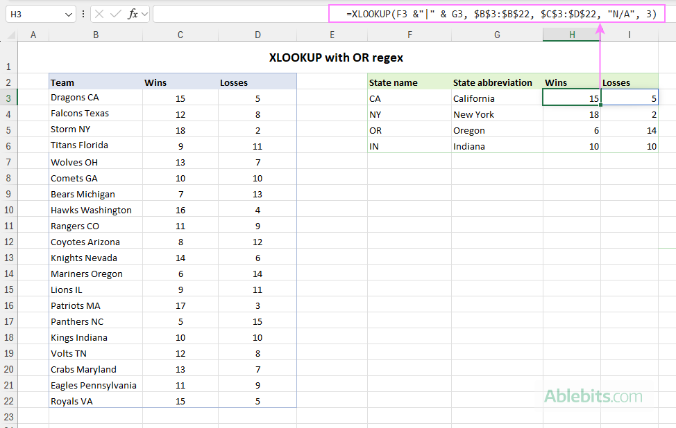
How this formula works:
- F3 & "|" & G3 creates a regex pattern like "NY|New York".
- match_mode = 3 tells XLOOKUP to use regex match.
- Excel checks each team name in B3:B22 for either NY or New York.
- When a match is found, the formula returns the number of wins from column C and losses from column D.
Formula B. XMATCH with OR regex
Next, sort your table by wins (column C) in descending order. The row order now reflects the ranking by wins: the team with the most wins is first, the next is second, and so on.
To find where the New York team stands in this ranking, use XMATCH with the same regex pattern:
=XMATCH("NY|New York", $B$3:$B$22, 3)
Or, you can use a dynamic regex pattern built from the abbreviation in F3 and full name in G3:
=XMATCH(F3 &"|" & G3, $B$3:$B$22, 3)
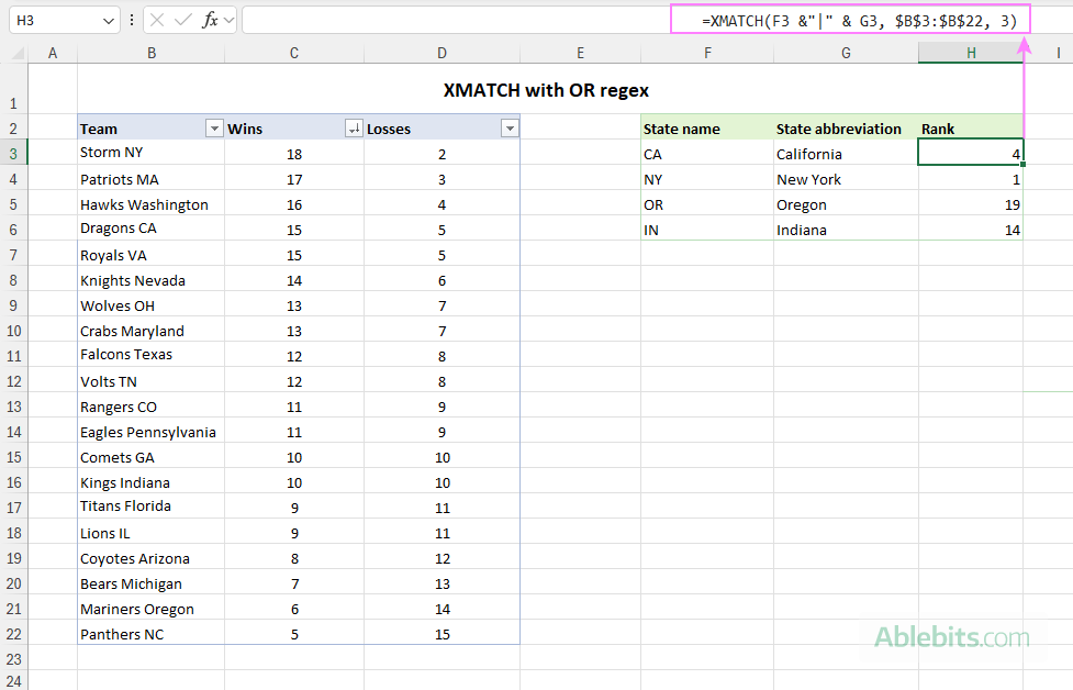
What the formula does:
- Looks for the first team name in B3:B22 that contains either the value in F3 or G3.
- Returns its position in the sorted list, which is the team's ranking by wins.
Example 3. XLOOKUP regex to match a separate word
There are times when you need to look up rows where a certain text appears as a standalone word, not just part of a bigger word. In the dataset below, column B contains product descriptions such as "chocolate bar" and "chocolatey topping". The purpose of this example is to return the product details where "chocolate" appears on its own.
To handle this, regex provides word boundaries, written as \b. These mark the edges of a full word and prevent matches inside longer words.
In our case, to match the word "chocolate", you can use the regex "\bchocolate\b" for the lookup value:
=XLOOKUP("\bchocolate\b", $B$3:$B$22, $C$3:$D$22, "", 3)
Or you can let the user type any word into F3 and build the pattern dynamically:
=XLOOKUP("\b" & F3 & "\b", $B$3:$B$22, $C$3:$D$22, "", 3)
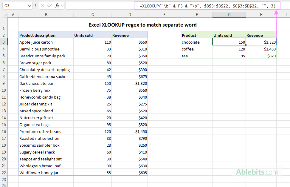
How this formula works:
- \b marks a word boundary, so the match must begin and end at a natural word break. For example, the formula matches "chocolate bar", but not "chocolatey topping".
- When a match is found, XLOOKUP returns the Units sold and Revenue values from columns C and D for the row where the F3 value appears as a separate word.
Example 4. XLOOKUP regex for case-insensitive match
Sometimes the word you are searching is written in different letter cases such as coffee, Coffee, or COFFEE. Because regular expressions are case-sensitive by nature, you need a way to match text regardless of how it is written. That can be done with the help of the inline case-insensitive modifier (?i).
In this example, column B contains product descriptions with a mix of uppercase and lowercase variations. Your task is to return the product details even when capitalization differs.
Let's say you want to find the first occurrence of coffee, no matter the text case. For that, just add the (?i) flag at the beginning of the regex pattern:
=XLOOKUP("(?i)coffee", $B$3:$B$22, $C$3:$D$22, "", 3)
This returns the Units sold and Revenue values for the product where coffee appears in any letter case, either on its own or as part of a bigger word.
And here is a dynamic version of the formula based on the value in F3:
=XLOOKUP("(?i)" & F3, $B$3:$B$22, $C$3:$D$22, "", 3)
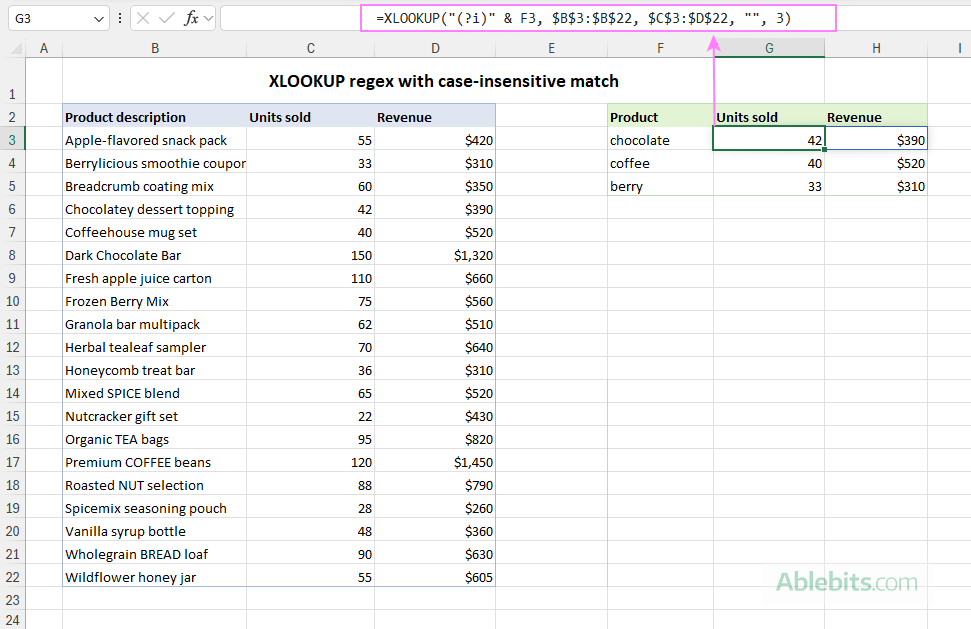
How this formula works:
- (?i) makes the match case-insensitive, so tea, Tea, and TEA all match.
- XLOOKUP searches column B using regex match mode and returns the values from columns C and D for the row containing the text typed in F3.
Regex match vs wildcard match in Excel
The XLOOKUP and XMATCH functions also support wildcards via match_mode = 2:
- * – any number of characters
- ? – any single character
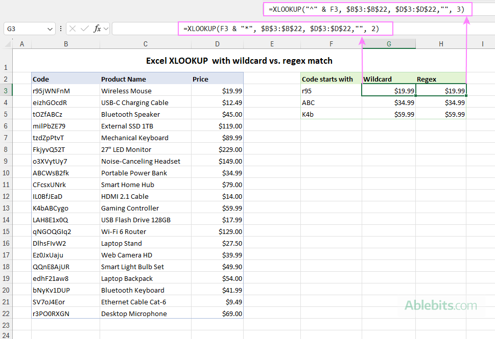
Simple partial matches that begin with, end with, or contain certain characters/text are often easier to perform with wildcards. For instance, to find a value that starts with "ABC", you can use this XLOOKUP formula with a wildcard match:
=XLOOKUP("ABC*", $B$3:$B$22, $D$3:$D$22, "", 2)
Though a regex match will also work:
=XLOOKUP("^ABC", $B$3:$B$22, $D$3:$D$22, "", 3)
The screenshot below shows the equivalent formulas built dynamically using the input values in F3:F5.
So, when do you actually need regex?
Regex becomes useful when you wish to:
- Match structured patterns, such as "3 letters, 2–4 digits, then 2 letters".
- Validate formats like IDs, phone numbers, and email addresses.
- Work with "this OR that" patterns using the | operator.
- Use anchors (^, $), word boundaries (\b), or character classes such as [0-9A-Za-z].
Whenever a pattern is too specific or complex for wildcards to express, regex is usually a more reliable option.
Practical tips on using regex match in Excel
The tips below highlight a few useful insights to keep in mind as you begin exploring regular expressions in Excel.
- XLOOKUP and XMATCH use PCRE2. Excel's regex implementation is based on PCRE2 (Perl-compatible regular expressions). That gives you access to a rich syntax and many online regex testing services that use the same flavor. If a pattern works in a PCRE2 tester, it will usually work in Excel.
- Use anchors and boundaries for precision. Patterns like ^ (start), $ (end), and \b (word boundary) help to match text exactly where you intend and avoid accidental false matches.
- Case sensitivity. Regex patterns are case-sensitive by default. To ignore case, add the inline modifier (?i) at the beginning of your pattern.
- Build patterns dynamically from cells. You rarely need to hardcode a full regex in Excel formulas. You can assemble pattern dynamically by including values from cells. This is especially handy when the user enters a variable part of the pattern (like a prefix or middle digits) in the input cell, while the rest of the structure stays fixed.
- Performance considerations. Regular expressions are more computationally intensive than exact or wildcard matches. On very large ranges, regex-based XLOOKUP or XMATCH formulas may take longer to calculate.
To improve performance:- Use range references such as A2:A100 instead of whole columns like A:A.
- Convert your data to an Excel table, then use structured references that expand automatically without scanning unnecessary rows.
- Avoid repeating the same complex regex calculation across dozens of cells if a helper column can do the same job.
Now that you know how to put regex match to work in Excel, you can start solving lookup problems that used to feel tricky. And when you are ready to practice, feel free to download the sample workbook below and experiment as much as you like.
Practice workbook for download
XLOOKUP and XMATCH with regex - formula examples (.xlsx file)
 by
by