 by
by The tutorial shows how to use the TRANSLATE function to convert text between more than 130 languages with a simple formula. You'll also discover how to use the built-in Microsoft Translator tool in Excel 365 - 2016.
If your Excel sheets contain product catalogs, multilingual reports, customer feedback, or other text that needs to be translated into different languages, you could copy it into an online translator one piece at a time. Or you can save yourself a lot of repetitive work by translating it dynamically with a formula right inside your Excel worksheet.
Excel TRANSLATE function
The TRANSLATE function in Excel converts text from one language to another. Unlike traditional text functions, it connects to online Microsoft Translation Services, so an internet connection is required.
TRANSLATE syntax
The syntax of the Excel TRANSLATE function is:
TRANSLATE(text, [source_language], [target_language])
Where:
- text – the text to translate. This can be a text value enclosed in quotation marks or a reference to a cell containing the text.
- source_language (optional) – the language code of the original text. If omitted, Excel attempts to detect the language automatically.
- target_language (optional) – the code of the language to translate into. If omitted, Excel uses your system language as the target language.
The TRANSLATE function is typically used for localizing product descriptions, international reporting, collaborating across multilingual teams, and other tasks that involve working with text in multiple languages.
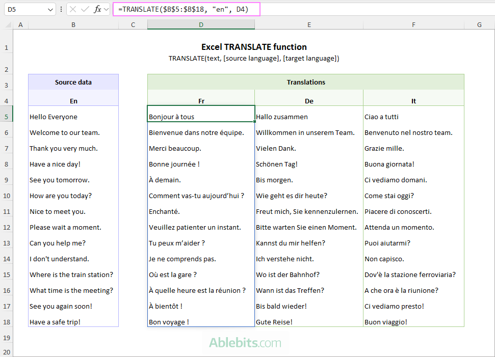
Usage notes:
- The function uses ISO language codes. For example, "en" for English, "es" for Spanish, "fr" for French, "de" for German, etc.
- Automatic language detection works for most, but not all, supported languages. For the most accurate translations, especially with short words or phrases, it's best to specify the source language whenever you know it.
- If the target language is not specified, Excel translates the text into the language defined in your operating system's Region settings.
- The function always returns text values, even if the source data is numeric.
- If the text argument refers to a blank cell, TRANSLATE returns an empty string ("").
- Because the function uses Microsoft Translation Services, an internet connection is required.
TRANSLATE function availability
The TRANSLATE function is available only in subscription-based versions of Excel:
- Excel for Microsoft 365 (Windows and Mac)
- Excel for mobile (iOS and Android)
It is not available in the standalone (perpetual) versions of Excel, including Excel 2024, Excel 2021, Excel 2019, and earlier.
Language codes
For the source_language and target_language arguments of the TRANSLATE function, you need to supply the language as a standard ISO language code. The function currently supports over 130 different languages.
Note that some languages have multiple writing systems or regional variants. For example, for Simplified Chinese the language code is "zh-Hans", while for Traditional Chinese it is "zh-Hant".
The table below lists some of the most commonly used language codes. For the complete list, see Supported Languages and Language Codes.
| Language | ISO Code | Language | ISO Code |
|---|---|---|---|
| Arabic | ar | Italian | it |
| Bengali | bn | Japanese | ja |
| Chinese (Simplified) | zh-Hans | Korean | ko |
| Chinese (Traditional) | zh-Hant | Polish | pl |
| Dutch | nl | Portuguese | pt |
| English | en | Russian | ru |
| French | fr | Spanish | es |
| German | de | Thai | th |
| Hindi | hi | Turkish | tr |
| Indonesian | id | Vietnamese | vi |
Tip. You don't have to memorize these codes. When entering a TRANSLATE formula in Excel, the AutoComplete feature displays a searchable list of supported languages, making it easy to find and insert the correct code.
How to translate in Excel with formula
Let's start with a basic example that shows how to translate a list of phrases from one language into another in Excel.
To build a TRANSLATE formula, you need to define three arguments: the source text, the source language, and the target language. While the last two are optional, specifying them explicitly usually produces the most accurate and predictable results.
Source text
You can supply the text to translate in two ways:
- Traditional one-formula-per-cell approach – reference a single cell and then copy the formula down:
=TRANSLATE(B3, "en", "fr") - Dynamic array approach – reference the entire range and let the translated results spill automatically:
=TRANSLATE(B3:B18, "en", "fr")
When translating a predefined list of values, the dynamic array approach is usually a better choice. It lets you do all translations in one go and eliminates the risk of accidentally overwriting or deleting a formula in one of the cells.
Source and target languages
In the above formulas:
- "en" specifies the source language (English).
- "fr" specifies the target language (French).
If you already know the language codes, simply type them directly into the formula enclosed in quotation marks.
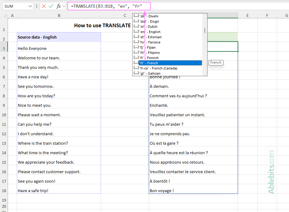
Alternatively, let Excel do the work by using Formula AutoComplete (aka IntelliSense) which suggests supported languages as you type:
- Begin typing the TRANSLATE formula.
- When you reach the source_language or target_language argument, Excel displays a drop-down list of supported languages.
- Double-click the desired language to insert its code into the formula automatically, complete with the required quotation marks.
TRANSLATE formula with automatic language detection
In theory, you can omit both the source_language and target_language arguments:
- If you leave out the source language, Excel tries to detect it automatically.
- If you omit the target language, the text is translated into your system language.
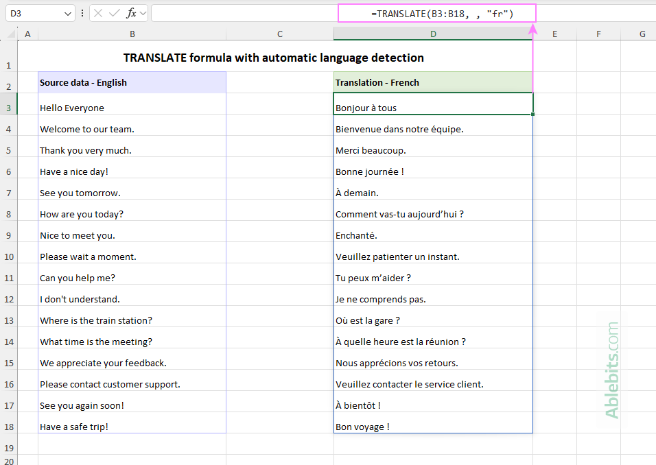
For example, the following formula lets Excel determine the original language:
=TRANSLATE(B3:B18, , "fr")
In our case, Excel has no problems with identifying the source language of all phrases (English) and translating them into French.
Automatic language detection is convenient when you're working with text in different languages or simply don't know the original language. However, if you do know it, it's usually best to specify the source_language argument. This helps Excel choose the correct translation, especially for short words or phrases that may exist in more than one language or have different meanings depending on the context.
Excel TRANSLATE formula examples
Now that you're familiar with the basics, let's look at a few practical examples that show different ways to use the TRANSLATE function in real-world scenarios.
Example 1: Excel formula to translate from English to Hindi
One of the biggest advantages of the TRANSLATE function is its ability to translate text into languages that use completely different alphabets or writing systems.
For example, you can translate your Excel data from English to Hindi even if you don't have a Devanagari keyboard installed on your computer. All you need to know is the standard language code for Hindi, which is "hi".
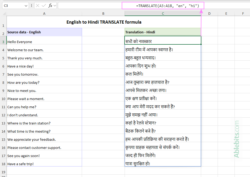
Assuming your English source data is in cells B3 through B18, you can translate the entire range using the following formula:
=TRANSLATE(A3:A18, "en", "hi")
The function translates each English phrase into Hindi and returns the results as a dynamic array.
Example 2: Translate to multiple languages with one formula
While the target_language argument of the TRANSLATE function natively expects a single input, you can still have it return translations in several languages at once. This can be achieved in two ways.
Method 1. Supply an array of language codes
Hardcode an array of target language codes directly into the formula by enclosing them in curly brackets like this:
=TRANSLATE(A3:A18, "en", {"de","es","it"})
Method 2. Reference a range with language codes
For a more dynamic setup, enter your target language codes into adjacent cells (e.g. a header row) and reference that specific range in your formula. For example:
=TRANSLATE(A3:A18, "en", C2:E2)
This approach is more flexible because you can add, remove, or change the target languages simply by editing the codes in the worksheet without modifying the formula itself.
In this example, both formulas translate the English item names in A3:A20 into German (de), Spanish (es), and Italian (it), returning the results in three adjacent spill columns.
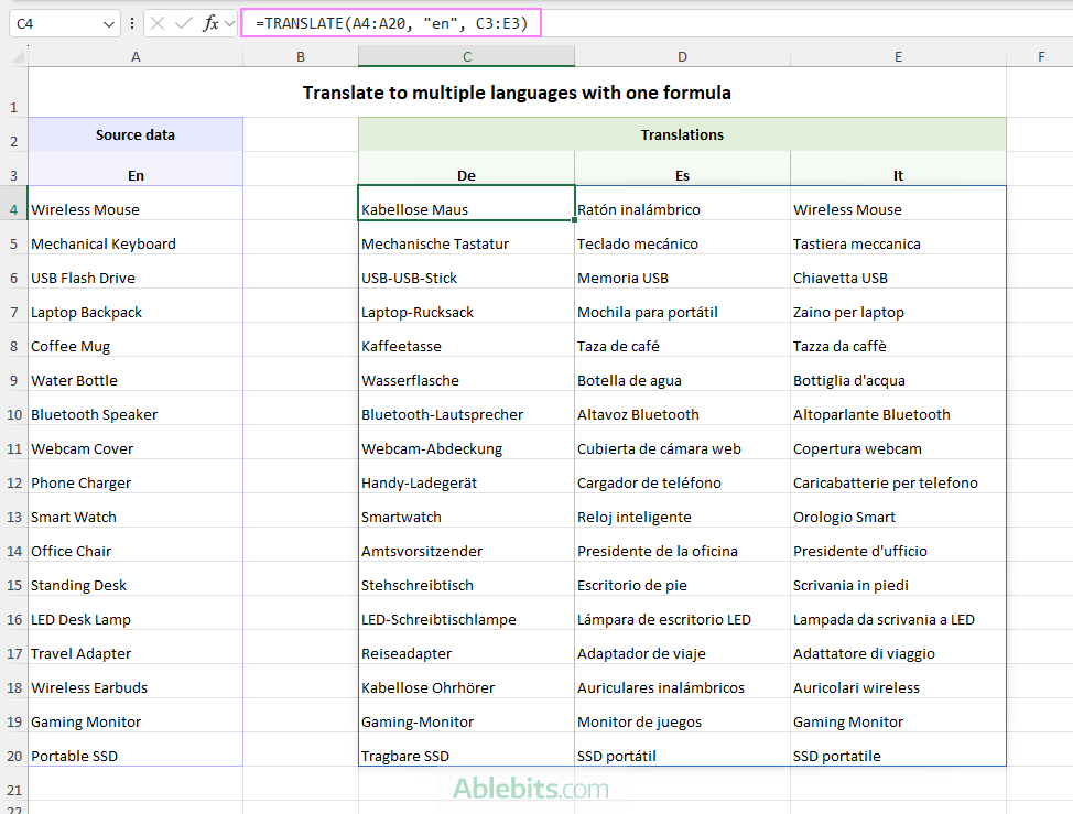
This multi-language approach is especially useful for preparing multilingual product catalogs, dynamic reports, software documentation, or other content that needs to be available in several languages.
Example 3: Translate dynamically based on dropdown language selection
This example shows how to translate text in Excel dynamically based on the language selected from a drop-down list.
Linking the TRANSLATE formula to a dropdown is a great way to create interactive worksheets, reports, or dashboards. Whenever a user picks a different language, the translations update automatically – no need to edit the formula.
Imagine you're building a dashboard for a customer service team, where support agents need standard responses translated instantly for customers around the world.
To set it up, you need 4 things: source phrases, a lookup table with language codes, a dropdown list for selecting the target language, and a TRANSLATE formula itself.
Step 1: Set up the worksheet
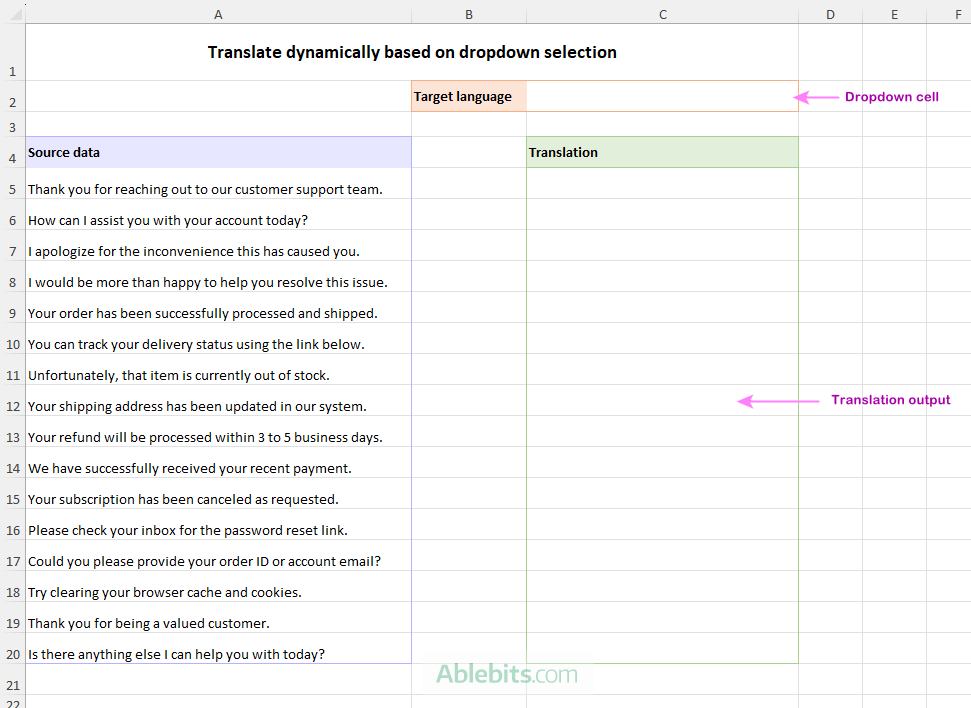
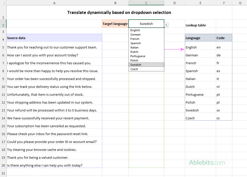
Start by organizing your worksheet. Enter the source text in one column (A5:A200, leave some cell for the target language selector (C2), and reserve a range for the translated results (C5:C20).
We'll populate the drop-down in the next step and use its selection to control the translation formula.
Step 2: Create a language lookup table
Create a lookup table somewhere on the worksheet, for example in E4:F14 that pairs each language with its code.
For a European e-commerce business, you could include these commonly supported languages:
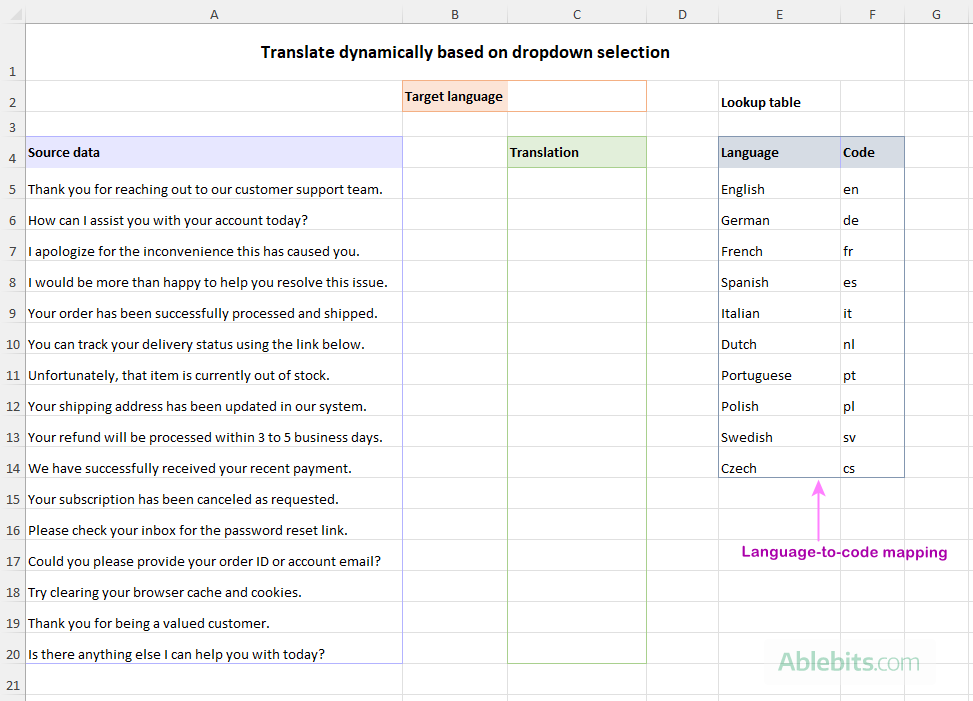
We'll use this table in the next steps to populate the drop-down list and retrieve the correct language code for the TRANSLATE formula.
Tip. We keep the lookup table on the same spreadsheet so it's easier to follow along. In real workbooks, it makes sense to place it on a separate sheet to avoid cluttering the main worksheet.
Step 3: Create a drop-down list
Now that you have the supported languages in a lookup table, it's time to let users choose the translation language from a drop-down list.
While you could create a regular drop-down, it's usually better to make it dynamic. That way, if you add or remove languages from the lookup table later, the drop-down updates automatically without any extra work.
In Excel 365, creating a dynamic drop-down is incredibly easy with the TRIMRANGE formula like this:
=TRIMRANGE($E5:$E20) Here, E5 is the first cell in the lookup table, and E20 is the last cell of the range you want to reserve for future language additions. TRIMRANGE automatically ignores any blank cells at the end of the range, so the drop-down contains only the languages that are currently listed.
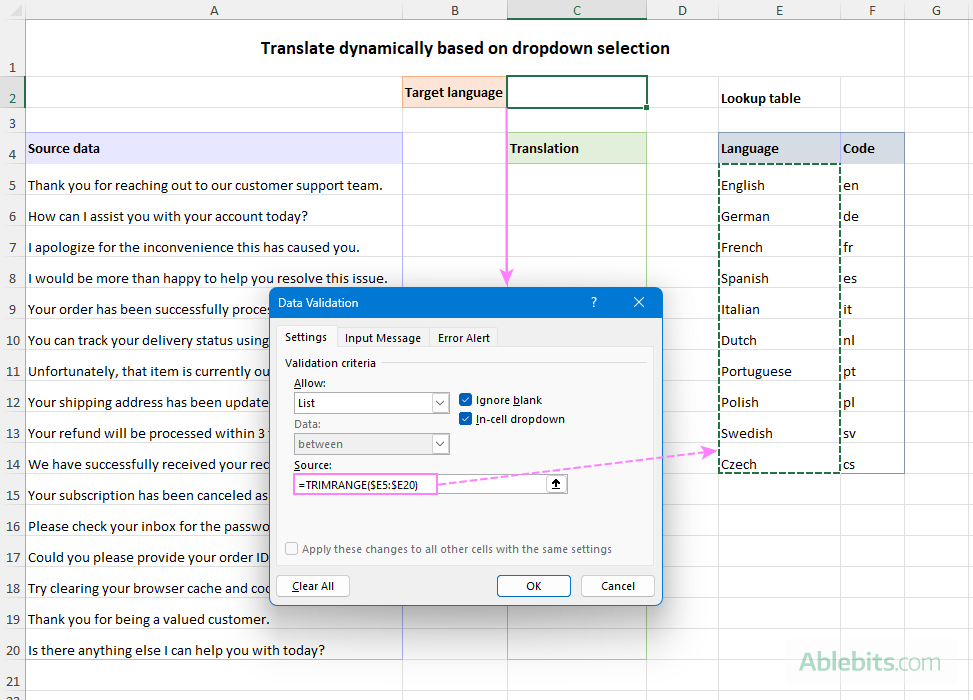
For the detailed instructions, see How to create a dynamic dropdown list in Excel.
The drop-down list is now ready to use. As you add new languages to the lookup table or remove existing ones, the list in C2 automatically expands or shrinks without adjusting the Data Validation settings.
Step 4: Write the TRANSLATE formula
With everything in place, all that's left is to write the formula that ties it all together. We'll use XLOOKUP to map the language selected in the drop-down to the corresponding language code, and then pass that code to the TRANSLATE function.
Enter the following formula in C5:
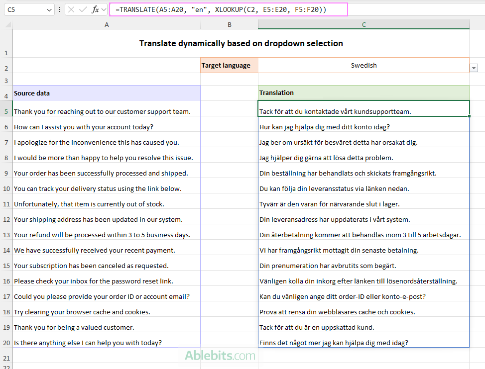
=TRANSLATE(A5:A20, "en", XLOOKUP(C2, E5:E20, F5:F20))
Here's how it works:
A5:A20contains the English product names."en"tells Excel that the source language is English.XLOOKUP(C2, E5:E20, F5:F20)looks up the language selected in C2 and returns the corresponding code from column F.
As soon as you select a language from the drop-down list, Excel translates all product names into that language. Simply choose a different language, and the translations update automatically.
Notice that the lookup and return ranges in XLOOKUP extend beyond the current data in the Lookup table. This is done intentionally to leave room for future additions.
Tip. To make this setup even easier to maintain, you can create dynamic named ranges for the language names and their corresponding codes, then supply those names in the XLOOKUP formula instead of range references.
Excel TRANSLATE function not working
If your TRANSLATE formula isn't returning the expected result, the cause is usually one of a few common issues. Here's what to check.
#NAME? error
A #NAME? error usually means Excel doesn't recognize the TRANSLATE function. This can happen if:
- The function name is misspelled.
- Your version of Excel doesn't support TRANSLATE. The function is available only in Excel for Microsoft 365 and Excel mobile.
#VALUE! error
A #VALUE! error most commonly indicates that one or both language codes used in the formula are invalid or not supported. To resolve the issue:
- Check that the
source_languageandtarget_languagearguments use valid ISO language codes. - Make sure the codes are enclosed in quotation marks, for example "en" or "fr".
- If you're using cell references, verify that the cells contain valid language codes without typos or non-printing characters.
#CONNECT! error
A #CONNECT! error means Excel couldn't connect to Microsoft Translation Services.
This usually happens when:
- Your computer isn't connected to the internet.
- Your network or firewall is blocking access to Microsoft's online services.
- The translation service is temporarily unavailable.
Check your internet connection and try recalculating the formula again after a few moments. If the problem persists, verify that Microsoft online services are accessible from your network.
Translate Excel sheet to another language with built-in Microsoft Translator
If the TRANSLATE function isn't available in your version of Excel, you can use the inbuilt Microsoft Translator tool. Although it doesn't translate text dynamically like a formula, it's still a quick option for translating selected cells.
Here is how to use it:
- Select the cells you want to translate.
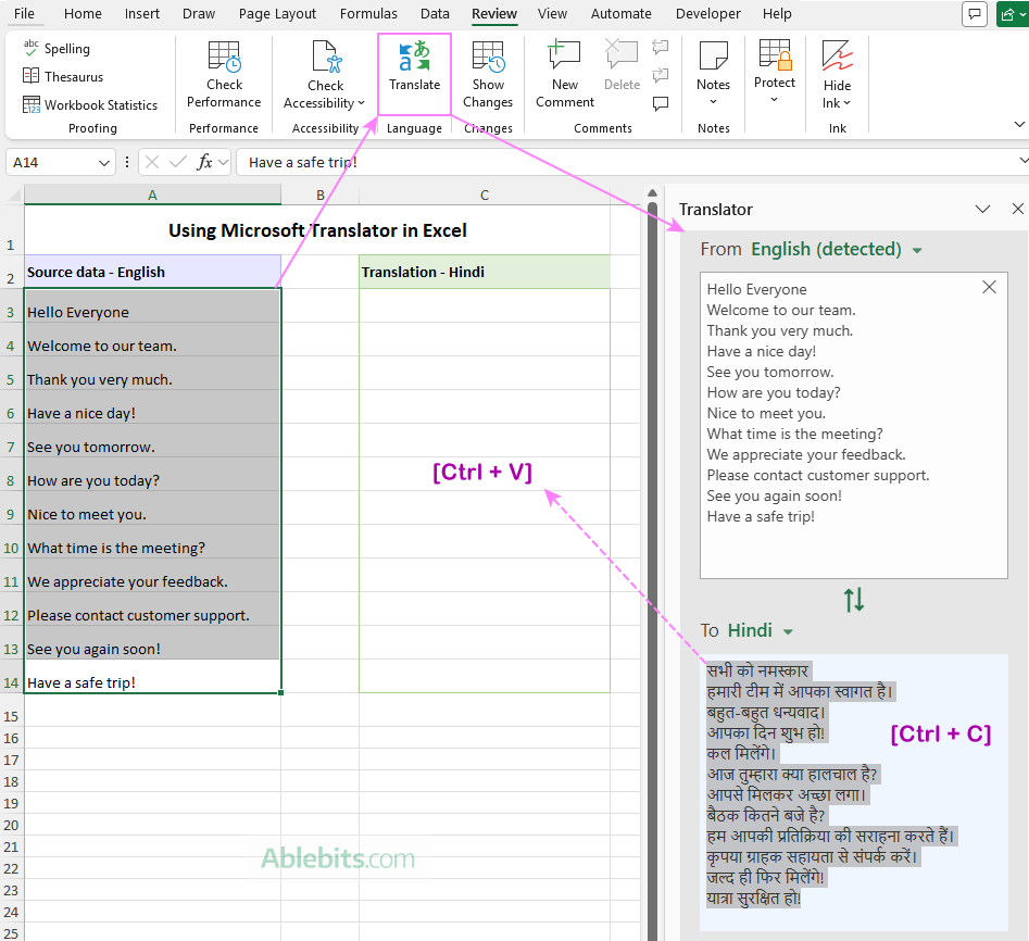
- On the Review tab, in the Language group, click Translate. The Translator pane opens on the right.
- In the From drop-down list, select the source language, or leave Auto-detect if Excel identifies it correctly.
- In the To drop-down list, choose the target language.
- Copy the translated text (Ctrl + C) and paste it back into your worksheet (Ctrl + V).
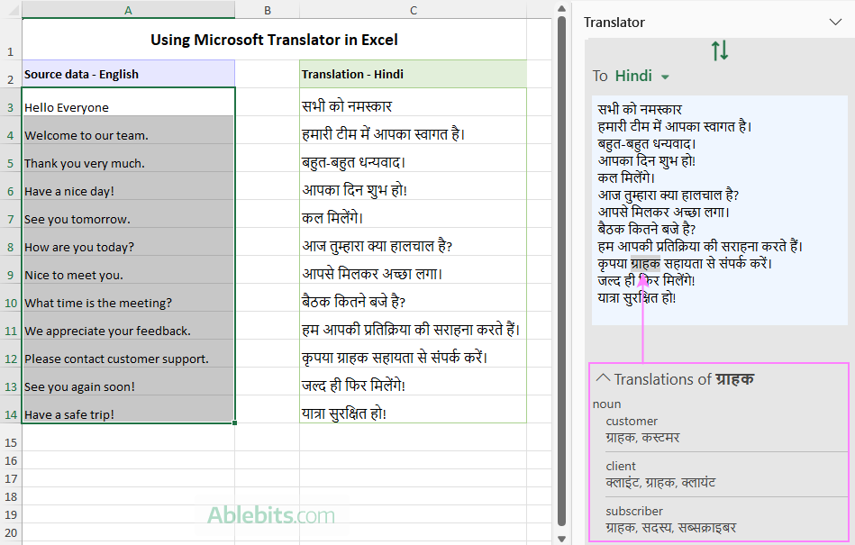
Compared to the TRANSLATE function, this method has a couple of drawbacks. Because the translated text is pasted as static values, it doesn't update automatically when the source text changes. If you edit the original data, you'll need to run the translation again and replace the existing results manually.
On the plus side, the Translator pane provides more than just the translated text. Hover over any specific word to see additional information such as alternative translations, meanings, and parts of speech. This can be especially helpful when you're translating individual words or short phrases and want to choose the most appropriate translation.
In conclusion: If your spreadsheets regularly cross language barriers, the TRANSLATE function is well worth adding to your Excel toolbox. It won't replace a professional translator, but for everyday work it's surprisingly capable, and much faster than translating one cell at a time.
Practice workbook for download
Excel TRANSLATE formula examples (.xlsx file)