Many tasks you perform in Excel involve comparing data in different cells. For this, Microsoft Excel provides six logical operators, which are also called comparison operators. This tutorial aims to help you understand the insight of Excel logical operators and write the most efficient formulas for your data analysis. Continue reading
Comments on: Excel logical operators: equal to, not equal to, greater than, less than
 by Svetlana Cheusheva, updated on
Comments page 3. Total comments: 717
Hi,
I am trying to calculate:
If A1 >A2 (by 10%) make A3 = 1
If A1 >A2 (by 20%) make A3 = 2
If A1 >A2 (by 30%) make A3 = 3
and so on?
Hello Burrod,
If I understand your task correctly, the following formula will do the trick:
=ROUNDUP((A1-A2) / A2*100, -1)/10
Hi,
If decimal in cell more than 0.20 = 0.50;
If decimal in cell more than 0.50 = 1;
If decimal in cell less than 0.20 = 0
How to workout with excel formula for a cell to match the above 3 things in order to get the result ??
Example :
USD 134.63 = USD 134.50;
USD 238.84 = USD 239
USD 73.19 = USD 73
Hey Lance,
You can do this with the following formula (with your value in cell A1):
=IF(A1 - TRUNC(A1) >0.5, 1, IF(A1 - TRUNC(A1) > 0.2, 0.5, 0))+ TRUNC(A1)
Hope this helps!
how do i write formula for...
if c21 is more than 40, multiply what is more than 40 by 15.00
So what happen if c21 is no greater that 40?. Well, below formula leave the c21 if it's not grater than 40
=If(c21>40,c21*15.00,c21)
i have this excel formula involving sumif with 2 columns, the test column is comprised of one letter having 3 possible values in column, the sum column has numbers
the formula is this =SUM(K13:K2005)/(SUMIF(J13:J2005, "", H13:H2005))
j colums is the test column with the letters, h is the value colums added with the numbers
my question is what "" means in this instance
please help
thank you
Hi Cristian,
"" means an empty string. In other words, your SUMIF function says: if a cell in column J is empty, then add up a number in column H in the same row.
Hi,
can you please explain how can i type greater than and less then symbol in excel formula or i have to download this symbol.
Regards
Abdul Wahab
Hi Abdul,
The 'greater than' and 'less than' symbols (also called angle brackets) are found on all computer keyboards. On U.S. keyboards, greater than (>) is usually located on the same key as the period and less than (<) on the same key as the comma.
WOW! It did it again....
Sorry for this. Our blog engine occasionally mangles formulas with "greater than" and "less than" operators, and our web-master can do nothing about it. Aargh...
It has been 20 years since I last took a boolean class...
I have a simple basic combination of IF(AND( >= to problems for you....
I am trying to make a simple entry to say: if the number in these three locations are ALL greater than 5 - then count it as one.
=IF(AND(B439>5,C439>5,D439>5),1,0) -
But here is the catch: I need zero to be counted as a ten place holder. So I need it to count all numbers in these locations which equal 6, 7, 8, 9, & 0.
At the other end of the stick - I also need it to count everything greater than 0 and less than 6. So I need it to count all numbers in these locations which equal 1, 2, 3, 4, & 5. Ignoring the zero...
But for some reason the combinations of Greater than and equal to refuse to give me the answer I need.... Help....
Can't seem to ever find the right examples of multiple combinations of nested Boolean...
I tried this - but it doesn't work:
=IF(AND(B435=0,B435>=6,C435=0,C435>=6,D435=0,D435>=6),1,0)
This does seem to work with the count 1 to 5:
=IF(AND(B435>=1,B435=1,C435=1,D435<=5),1,0)
Not sure what th difference is - but there must be one. The bottom one works and the top one does not...
MANY MANY THANKS! I was trying all kinds of versions - even played with NOT commands nothing worked. Your solution is GOD send.
Hi Steven,
The difference is that the logical test in the first formula can never be TRUE because a number cannot be equal to 0 and greater than 6 at the same time :)
You need a combination of OR and AND statements in this case:
=IF(AND(OR(B435=0,B435>=6), OR(C435=0,C435>=6), OR(D435=0,D435>=6)), 1, 0)
My case is for my item analysis in school.
E.g. 35 students in a class
The table says if:
75% above of the class size is M
<75% to 50% of the class size is NM
<50% below of the class size is LM
Can you help me to create a formula for this case. Thank you.
Hello, James,
Please try the following formula:
=IF(A1 >= 75%, "M", IF(A1 >= 50%, "NM", "LM"))
You can learn more about Nested IF function in Excel in this article on our blog.
Hope you’ll find this information helpful.
I need a formula that figures out how many entries in a range and then divides by that about of entries. Example if A1= 0, A2, = 3, A4=5 then divide by 2.
Thank you for your help. I actually have 7 entries - 1 for each day of the week, and want to divide only by the days that actually have a number greater than 0. So what I need is the sum of the 7 days then divide by only the number that had an actual value greater than 0.
Thank you!
Hi Pauline, I hope you already received a response, but if not here's my answer. You would use the Countif function. It would look like this:
=COUNTIF(B1:B3,">0") the function looks at the cells B1 to B3 and returns a number between 0 and 3 depending on how many of the cells have a value higher than 0.
Que. If A1>B1 & C1=D1 then bonus will be (A1*0.002), but If A1>B1 & C1=D1 and F1>G1 & H1=I1 then bonus will be ((A1+F1)*0.002*2). Please suggest correct formula to be used?
Hello, a formula that would work for you is the following:
=IF(AND(A1>B1, C1=D1, F1>G1, H1=I1), ((A1+F1)*0.002*2), IF(AND(A1>B1, C1=D1), A1*0.002, 0))
I used the information from https://www.ablebits.com/office-addins-blog/excel-nested-if-statement/ to help come up with this answer.
Hi,
I have a set of number in a columns from 12 to 30 & I want result for them in 2 word
that can be more than 15 or less than 15. Is there a way I can get a formula result for these number. thank you
Abdul:
If I understand your question an IF THEN OTHERWISE statement will work for you. Where the first number is in A2 enter this in B2:
=IF(A2<15,"Less Than 15","More Than 15")
It says, if the value in A2 is less than 15 then display "Less Than 15" otherwise display "More Than 15".
I applied a formula like
=A1
then it shows whatever is there in A1 . But if A1 is blank then its showing 0 instead of blank.
I want it blank if it is blank in A1
Hello, Manu.
Please try to apply the formula below instead:
=IF(ISBLANK(A1), "", A1)
Hope this is what you need.
IF(E8>60<90,F8,0)
THIS FORMULA NOT GIVEING MY ANSWER
Hello, Amit,
Please try the following formula:
=IF((AND(E8>60, E8<90)), F8, 0)
Please also have a look at the following article on our blog:
Excel IF statement with multiple AND/OR conditions
Hope you'll find this information helpful.
=IF((AND(E8>60, E84,R5<=4)),AE5,VLOOKUP(AE5,VALIDATION!$M$3:$P$24,4))
great
I have an IF statement that looks at one cell and depending on what "class code" I have in that cell it refers to another cell then adds that number into the calculation. This is working fine but I want it to then put 0 instead of a negative number. I tried adding If(<0,0,) but it is not working and I have tried several variations of less than zero. Any suggestions?
Malissa:
Can you post the formula that was working?
21080931
21079882
21079117
21080035
21234
21225
22225
21228
I WANT TO ADD DOT (.)AFTER 2 NUMBERWHICH LEN IS GREATER THAN 6 NO
AND WHICH IS SMALLER THAN 5NO ADD ONLY 1 DOT (.)AFTER THE VERY FIRST 2 NO. PLEASE HELP ME
EX=
21.07.98
21.07.9117
21.08.0035
21.234
21.225
22.225
21.228
21080931 =IF((LEN(A1)<6),LEFT(A1,2)&"."&MID(A1,3,20),LEFT(A1,2)&"."&MID(A1,3,2)&"."&MID(A1,5,20))
HELP ME WITH THIS; =IF(A4>=14500+A4),IF(A4<14500+0
Evarist:
The statement in this cell is incomplete.
Right now it says, If A4 is greater than or equal to 14,500 + A4 or if A4 is less than 14,500 and this is as far as the statement goes.
What do you want to display in this cell?
What are you trying to say with the statement?
=(PROJECT.xlsx!WWC51_DOM)
trying to use another sheet as a reference while using the a cell from the original sheet to dictate which cell data from the other sheet to pull.
=(PROJECT.xlsx!('[ACESII Kit Time Change 1574.xlsx]sheet1'$A$1)_DOM)
-project is the 2ed sheet
-acesii time change is the original sheet. *this sheet is the sheet the formula will be placed in.*
-the "_dom" is the last four characters of each cell name in the 2ed data sheet. ex (wwc51_dom) (wwc21_dom)
- the second formula is the one i came up with but it isn't working. what i want is to use a cell from the original excel sheet to be my (WWC#), so that when i change the cell with the (WWC#) the formula placed on a different cell within the original sheet will display the WWC# information from the 2ed sheet.
ex: cell will read WWC51_DOM *DATE* / when i change the WWC# to WWC21_DOM, it'll pull WWC21 dates.
-1st & 2ed sheets are different excel documents
-sorry for the complicated question if theres a better way or if you could fix this it'd be greatly appreciated. Thanks
Danny:
I think what you're trying to accomplish can be done via a VLOOKUP formula.
Take a look at the articles here on AbleBits dealing with VLOOKUP or even INDEX/MATCH and see what you think.
If you need help after that post another question with some sample data if you can.
I'm working on performance review spreadsheets and I need a formula that will show me:
If >1 but 2 but <3 "Inconsistent to Proficient" and if = 2 ""Inconsistent" and if =3 then "Proficient"
Jasmine:
The logic isn't clear.
Both 2 and 3 are greater than 1, so the formula will break.
Should the first statement be:
If cell value =1 then "Inconsistent to Proficient" ?
Is there a score greater than 1 but less than 3 that is not 2?
Do not know why it cut some of question. The formula gives a false positive, need the formula to meet both requirements, not one.
=IF(OR(D4>10000,D420%,E4<-20%),"Amendment Required","No Amendment required")
Hello, OJ:
You've posted two similar but different questions which one contains the correct logic you want to use?
How do I set negative numbers in an IF function in excel? For example =IF(BK2-1)
Elissa:
Enter a negative number in a formula by enclosing it in a parenthesis, like this:
=IF(A133<=(-1),"Neg","Pos")
I have a problem, can you please assist.
I need to calculate a value,
Thus in words " if value A > value B and value A < value C; Return value D. This then needs to compare with 10 similar logical arguments, but only one answer can be correct.
How should my formula look like if the only constant is value A.
Regards
Andre:
Not exactly sure what you're looking for, but here's how you find the first part of your question. Where the values are in columns A through E.
=IF(AND(A1>B1,A1<C1),D1,E1)
In words this formula says, "If A1 is greater than B1 and A1 is less than C1 then return D1 otherwise return E1."
This is as far as I can follow your question.
Please give me formula of 10x5= 50
Hey Joser
You should write =10*5 and press enter
Thanks
Here we go - I have a simple formula that I am using:
=IF(F2>=K2,"yes","no")
What I need is to make K2 a constant. I've tried making it an absolute (ABS), but I think I'm just not putting it in the right place in the equation. One, it's a fixed number in the spreadsheet, and two, it will prevent the formula from going to K3,K4,K5,etc as I pull it down.
Any help would be great.
-PK
Hi!
Why not simply use an absolute reference? :)
=IF(F2>=$K$2,"yes","no")
Aha! I got it figured out. I was trying too hard. Thanks, though!
Hi,
If A5 is less than 10 then value become in B5 should be 0
And if If A6 is 11 then value become in B6 should be 50
And if A7 is 12 then value becomes in B7 is 100.
Please help.
Hi Vishal,
This can be done by using nested IFs. Please check out this article for the detailed explanation and formula examples:
Using nested IFs in Excel
I want to learn a formula for
if A1 is greater then B1 then show the result in C1 and but A1 is less than B1 than 0 or Nill will show in C1
i am trying
=if(A1>B1,A1-B1,Nill)
But its not working
Could you help me out.
Thanks In Advance
Hi Noor,
Please put the text value in your formula in double quotes or replace it with 0, i.e.:
=IF(A3>B3,A3-B3,"Nill")
Or
=IF(A3>B3,A3-B3,0)
Hope this will help.
I have a question. I want an Excel sheet to give me this.
In my cell I am subtracting A5-A6. If the answer is less than 60, I want to return 0. If it is 60 or more, I want the correct subtraction. How do I do that?
Hello,
Please try the following formula:
=IF(A5-A6<60, 0, A5-A6)
Hope it will help you.
Hi, this is probably an easy one for you but I can't get it right. If the cells A2-A11 have the value of B2 to display the value in C2. If the cells do not have the value from B2 the cells should be blank. I have the formula =IF(A2:A11=B2,"C2"," "). What am I doing wrong?
Hello,
If I understand your task correctly, please try the following formula:
=IF(ISERROR(MATCH(B2,A2:A11,0)),"",C2)
Hope this will help.
Hello Team,
I have Name in Column A, Mahesh, Suresh, Kailash, i.e. &
in column B I have count of their process order count i.e. 20, 30. 40, 0
I have 4 sheets (1-Dec, 2-Dec, 3-Dec) which is mentioned their name
I want total individual count in 5th Sheet by their name
Condition, it should not count if there is zero value, i.e. "0"
Hello,
If I understand your task correctly, please try to do the following:
1. Supposing that your cell A1 on the 5th sheet contains one of the names: Mahesh, Suresh, Kailash, etc.
2. Enter the following formula in cell B1 on the 5th sheet:
=IF(OR(VLOOKUP(A1,'1-Dec'!A:B,2)=0,VLOOKUP(A1,'2-Dec'!A:B,2)=0,VLOOKUP(A1,'3-Dec'!A:B,2)=0,VLOOKUP(A1,'4-Dec'!A:B,2)=0),"",(VLOOKUP(A1,'1-Dec'!A:B,2)+VLOOKUP(A1,'2-Dec'!A:B,2)+VLOOKUP(A1,'3-Dec'!A:B,2)+VLOOKUP(A1,'4-Dec'!A:B,2)))
Hope this will help you with your task.
Dear Sir,
I have two columns of text, I understand how to find exact matches through =IF(A2=B2, "Match","No Match") but how can I find partial matches. Such as A1 = "Patient has Sepsis" and B2 = "Sepsis" how can I still report this as a Match when the text is not an exact 100% match? If any text in A1 is found in B1 it should be reported as a Match.
Thank you for your help,
S
Hello,
If I understand your task correctly, please try the following formula:
=IF(LEN(SUBSTITUTE(LOWER(A2),LOWER(B2),""))<>LEN(A2), "Match","No Match")
Hope it will help you.
kindly tell me how to write this in excel:
1)greater than 20 and less than 25?
2)greater than or equal to 20 and less than or equal to 25?
Hello,
If I understand your task correctly, please try the following formulas:
=IF(AND(A1>20,A1<25),"yes","no")
=IF(AND(A1>=20,A1<=25),"yes","no")
Hope it will help you.
Hi,
I am trying to apply a formula to find the greater then:
C2 = 335
B2 = 337.5/330.2
=IF(C2>Right(B2,Find("/",B2)-1),"True","False")
The output is not matching to the logic i am looking for as it giving "False"
Could you please help me?
Thanks
Hello,
Please try the following formula:
=IF(C2>VALUE(RIGHT(B2,LEN(B2)-FIND("/",B2))),"True","False")
Hope it will help you.
Hello,
I am trying to enter formula into excel to match below:
> 95% equals 5
90% - 94.9% equals 4
85% - 84.9% equals 3
75 - 85% equals 2
<75% equals 1
Could you pleased help me?
Thanks
Hello,
Please try the following formula:
=IFS(A1>95%,5,A1>=90%,4,A1>=85%,3,A1>=75%,2,A1<75%,1)
Hope it will help you.
Please i need a formula for the statement bellow
if value in cell A6 90 & 100 & 110 & =120 print 100%.
I write is like this =IF(10090,"80%",IF(110100,"90%",IF(120110,"95%",IF(I6>=120,"100%","0"%)))) but is not giving me what i need.
Please I will appreciate your input.
Hello,
If I understand your task correctly, please try the following formula:
=IF(A6>=120,"100%",IF(A6>=110,"95%",IF(A6>=100,"90%",IF(A6>=90,"80%","0%"))))
Hope this will work for you
Gross Pay Deduction
Up to 5,999 150
6,000 - 7,999 300
8,000 - 11,999 400
12,000 - 14,999 500
15,000 - 19,999 600
20,000 - 24,999 750
25,000 - 29,999 850
30,000 - 34,999 900
35,000 and above 1000
How to calculate by using IF formula in Excel please help
thank you
Hello,
Please try the following formula:
=IF(A1>=35000,1000,IF(A1>=30000,900,IF(A1>=25000,850,IF(A1>=20000,750,IF(A1>=15000,600,IF(A1>=12000,500,IF(A1>=8000,400,IF(A1>=6000,300,150))))))))
Hope it will help you.
i know this is probably a simple formula that i am just drawing a blank on but i need some help please. if cell A is not equal to $4 i need cell B to make up the difference. But if cell A is equal to or higher i need nothing to show up, cant have any negative numbers.
more information to help you: cell A is already formulated to be the sum of several other amounts, but if that cell does not equal $4 i need an adjustment cell to make up the difference.
Hi Arlene,
If my understanding of the task is correct, the following formula should work a treat:
=IF(A1<4, 4-A1, "")
I've done this heaps of times before but for some reason I'm struggling today. So, if I want to check if apples <= 10, then flag as"Too Low" or if oranges <= 20, then "Too Low" or if Pineapples <= 30 then "Too Low" The fruit names are in one column and the amounts in the other. I'm trying to string it all together and flag. If anyone can tell me that would be great.
Hello, Vicki,
Please try the following formula:
=IF(AND(A1="apples",B1<=10),"Too Low", IF(AND(A1="oranges",B1<=20),"Too Low",IF(AND(A1="pineapples",B1<=30),"Too Low","")))
Hope it will help you.
Hello Svetlana Cheusheva!
Your efforts to help students/employees concerning excel formulas are really appreciable.
I need to know formula for the below statement:
If we have a column having total marks of students like 60,75,25,115,150,250 etc and I want to show the grades int he next column in front of these values their grades like if less than 50 it is Fail, greater than 50 it is Fair, greater than 100 it is Good, greater than 200 it is Excellent.
Kindly guide me to write formula.
Thanks
Hi Sheraz,
This can be done with a classic nested IFs formula like this:
=IF(A2>200, "Excellent", IF(A2>100, "Good", IF(A2>50, "Fair", "Fail")))
thanx alot! :)
I meant >=16 then.........
Hello, David,
it looks like you could use conditional formatting with IF function.
You can read more about the rules of conditional formatting in this article.
If you don't know how IF function works, feel free to learn its usage here.
Hope you'll find what you need!
Hi,
Column D E
1 C1
2 C2
3 C3
4 C2
5 C3
6 C4
7 C5
8 C6
I want to put the value in column E if C1=10, C2= 20, C=30, C4= 40, C5= 60, C6= 70. What will be the formula??. I tried by using IF(OR fomula but failed. Would you help me?
Hi, Mehedi,
nested IF is exactly what you need. Please take a look at this tutorial to see how it works.
I have a formula that determines if a date is within a date range.
I want it to be TRUE IF the date falls between a selected start and end date, as well as IF they start and end date is the same date.
I'm using the AND function, to determine if it's equal to or greater than the start date, AND equal to or less than the end date.
=AND('Form Responses 1'!$A8>=$A$4,'Form Responses 1'!$A8 and <, correct?
not working
Dear fren,
can u all help me for this formula? even the result below -15% and above 15%, its follow the condition at range 10%.
=IF(AND((-10%)>=Z10=Z10>(-10.001%)),"NEED IMPROVEMENT",IF(AND((-100%)<=Z10<(-15.001%)),"BAD",IF(AND(1%<Z10<=10%),"GOOD",IF(AND(10%<Z1015%,"BAD",FALSE))))))
thanks
(-0.001%) to (-10%) GOOD
(-10.001%) to (-15%) NEED IMPROVEMENT
>(-15.001%) BAD
0% to 10% GOOD
10.001% to 15% NEED IMPROVEMENT
>15.001% BAD
I am trying to find out a formula for this one
eg :
1st 2nd 3rd 4th 5th 6th 7th
21.80 61.40 120.80 200.00 299.00 417.80 556.40
if answer has come greater than 300, value should '0'
in this eg 6th & 7th one should 0.
if it is come less than 300, value should true value, like 21.8, 61.4, 120.80
so please help me
1st = 21.8
2 = 61.40
3 = 120.8
4 = 200
5 = 299
6 = 417.8
7 = 556.4
how can we write this in excel formula "All student whose mark is more than 200 and less than 250 label it as “average” ".
Hi Sheryl,
we'll keep it simple-
Assume Column A is the students name and Column B contains their grade.
in C1 type;
=IF(AND(D3>200,D3<250),"Average","")"
Hope this helps!
HI,
I am making a spread sheet for conditional formula with if function.
if A10=250 and B10= opc (or Any text) then write specific number in third cell C10
Example: A10 = 250 , B10 = OPC or (Any text) , C10 = 170
Formula =if(A10=250 & B10=OPC,"170","0")
Actually i have cement Weight 250 in Cell A10 and Cement Type in OPC in Cell B10 Now i want that if i write 250 in Cell A10 and OPc in Cell B10 Then Right Price exact 170 in Cell C10
can you give me formula or any solution plz.
Hi, Usman,
Try this one in C10:
=IF(AND(A10=250,OR(B10="OPC",ISTEXT(B10))),170,0)
Hope it helps.
Thanks its works
You're welcome!
Hello, I need help to compare two cells like this. Want to compare cell B1 to A1 and soo on and I need to count every equal result, every A smaller then B and every B smaller then A.
A B Miks S = 1 Result
Miks M = 2 A = B = ?
Miks M Miks L Miks L = 3 A B = ?
Miks S Miks S
Miks L Miks M
A B
Miks M - Miks L
Miks L - Miks M
Miks S - Miks S
Miks S - Miks L
Miks S = 1
Miks M = 2
Miks L = 3
Need to count every equal, smaller and bigger.
A = B = ?
A B = ?
Hello! I have read through many of the comments and have a question:
I am working on a spreadsheet and if the number of years is equal to 0, I need it to be a value, if the number is between 1 and 5 I need a value, if it is 6 to 10 I need a value and if it is 10 to 15 I need a value. Can you help me figure this out?
=0 = $10.50
1 to 5 = $10.75
6 to 10 = $11.15
10 to 15 = $12.75
Thanks so much
You have to use the AND function, so something like =IFS((A1=>1)AND(A1<=5)),10.75), etc.
I have a similar issue but I need it to be if zero equals A5, if 1-5 equals B5, if 6-10 equals C5 and 10+ equals D5.
Can I do the ranges of numbers/years and have the formula grab the answer from calculations in the other cells?
I have the following formula and Excel continues to give me errors. Help, please!
=IF(B126>20,"A",IF(AND(B126=0),"B",IF(AND(B126(-20)), "C"), IF(B126<(-20), "D")))
Hello, Matthew,
first of all, you don't need to use AND function because you specify only one criterion after it. Then, you missed the logical operator in B126(-20): should B126 be equal to -20? Also, there's no need to use round brackets for negatives in this case.
So, try this formula:
=IF(B126>20,"A",IF(B126=0,"B",IF(B126=-20,"C",IF(B126<-20,"D")))) Please note that you didn't specify what to return when B126<0 but greater than -20; when B126=20 and when B126>0 but lower than 20. Logically the formula requires these criteria too.
But I do hope that the formula above is what you were looking for :)
Hi Svetlana,
Scenario:
F8 = 1
D10 = 0
E10 = 7
I want to create an IF formula to ask if F8 is greater than D10 but less than E10, then return a value of 1. If not, then return a blank.
I created the following:
IF(F8>D10<=E10,1,"")
but this returns a blank instead of 1. I am not sure why.
I am sure it is probably quite simple, but can't seem to solve it - I would be grateful for your help.
Many thanks!
Hi Aron,
you need to use AND in the condition of your formula. Try the following:Excel IF tutorial.
=IF(AND(F8>D10,F8
Help! I trying to find if cell A1 is equal to B1 and if it is highlight it a secific color, red. There are about 15k so I'll need to drag the formula down. Please help!
Hello, Anna,
if I understand your task correctly and you need to fill the cells with a colour depending on the result of the formula, then conditional formatting is what you need to take a look at.
You create the following rule:
=$A1=$B1
and apply it to
=$A:$B
Hope this helps.
Hi,
I am trying to apply a formula that returns a Text answer to the greater or less than number difference compared to an adjacent cell.
The purpose is for a 14 question questionnaire with either an A. or B. answer. The answer is determined by the criteria as follows:
"To score your test, add the number of questions you answered A and the
number you answered B"
- If your number of A answers is 3 or more than B answers, you are a
Protein Type.
- If your number of A and B answers are tied or within 2 of each other, you
are a Mixed Type.
- If your number of B answers is 3 or more than A answers, you are a
Carbohydrate Type.
I would like to return the text either "Protein Type", "Carb Type", "Mixed Type" based on the A. and B. totals.
Many Thanks
Hi Brad,
Let's assume that your data is arranged in the following way:
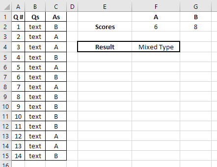
A1:C15 is the table with questions (Qs) and answers (As).
Using COUNTIF in F2 and G2 we can find out the number of 'A' and 'B' answers accordingly:
=COUNTIF(C2:C15,"A") (for F2)
=COUNTIF(C2:C15,"B") (for G2)
Then, in F4 we need to use nested IF function to apply all the conditions you described:
=IF((F2-G2)>=3, "Protein Type", IF(AND((F2-G2)<=2,(F2-G2)>=-2),"Mixed Type","Carb Type"))
or a bit shorter version:
=IF((F2-G2)>=3, "Protein Type", IF(ABS(F2-G2)<=2,"Mixed Type","Carb Type"))
Try to adjust this example formulas to your data, and learn more on the used functions from the links above. Hope it helps!