The tutorial shows how to extract number from various text strings in Excel by using formulas and the Extract tool.
When it comes to extracting part of a text string of a given length, Excel provides three Substring functions (Left, Right and Mid) to quickly handle the task. When it comes to extracting numbers from an alphanumeric string, Microsoft Excel provides… nothing.
To get a number from a string in Excel, it takes a little ingenuity, a bit of patience, and a bunch of different functions nested into each other. Or, you can run the Extract tool and have the job done with a mouse click. Below you will find full details on both methods.
How to extract number from the end of text string
When you have a column of alphanumeric strings where number comes after text, you can use the following formula to get it.
We will dwell on the formula's logic a bit later. For now, simply replace cell with a reference to the cell containing the original string (A2 in our case), and enter the formula in any empty cell in the same row, say in B2:
=RIGHT(A2, LEN(A2) - MAX(IF(ISNUMBER(MID(A2, ROW(INDIRECT("1:"&LEN(A2))), 1) *1)=FALSE, ROW(INDIRECT("1:"&LEN(A2))), 0)))
This formula gets number only from the end. If a string also has numbers in the beginning or middle, they are ignored:
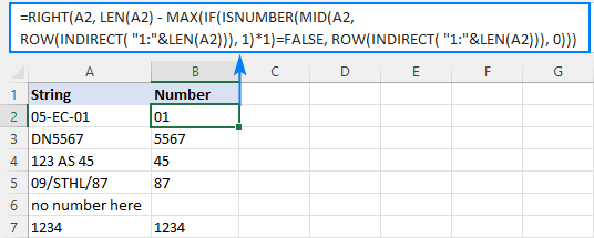
The extraction is performed with the RIGHT function that belongs to the category of Text functions. The output of this function is always text. In our case, the result is a numeric substring, which in terms of Excel is also text, not number.
If you need the result to be a number (that you can use in further calculations), then wrap the formula into the VALUE function or perform an arithmetic operation that does not change the result, say, multiply by 1 or add 0. To catch errors in the strings that do not contain a single number, use the IFERROR function. For example:
=IFERROR(VALUE(RIGHT(A2, LEN(A2) - MAX(IF(ISNUMBER(MID(A2, ROW(INDIRECT("1:"&LEN(A2))), 1)*1)=FALSE, ROW(INDIRECT("1:"&LEN(A2))), 0)))), "")
or
=IFERROR(RIGHT(A2, LEN(A2) - MAX(IF(ISNUMBER(MID(A2, ROW(INDIRECT("1:"&LEN(A2))), 1) *1)=FALSE, ROW(INDIRECT("1:"&LEN(A2))), 0))) +0, "")
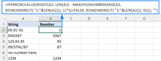
Note. In Dynamic Array Excel (Office 365 and 2021), you enter the formula in the usual way with the Enter key. In Excel 2019 and earlier, it only works as an array formula, so remember to press Ctrl + Shift + Enter to complete it.
How this formula works:
To extract number from an alphanumeric string, the first thing you need to know is where to start the extraction. The position of the last non-numeric character in a string is determined with the help of this tricky formula:
MAX(IF(ISNUMBER(MID(A2, ROW(INDIRECT("1:"&LEN(A2))), 1)*1)=FALSE, ROW(INDIRECT("1:"&LEN(A2))), 0))
To understand the logic, let's investigate it from the inside:
The ROW(INDIRECT("1:"&LEN(A2))) combination creates a sequence of numbers corresponding to the total of characters in the source string (A2), and we serve these sequential numbers to MID as the starting numbers:
MID(A2, {1;2;3;4;5;6;7;8}, 1)
The MID function pulls each individual character from A2 and returns them as an array:
{"0";"5";"-";"E";"C";"-";"0";"1"}
As MID is a text function, its output is always text (as you can notice, all the characters are enclosed in quotation marks). To turn numeric ones into numbers, we multiply the array by 1 (double negation --MID() will have the same effect). The result of this operation is an array of numbers and #VALUE! errors representing non-numeric characters:
ISNUMBER({0;5;#VALUE!;#VALUE!;#VALUE!;#VALUE!;0;1})
The ISNUMBER function evaluates each element of the array and gives its verdict in the form of Boolean values - TRUE for numbers, FALSE for anything else:
{TRUE;TRUE;FALSE;FALSE;FALSE;FALSE;TRUE;TRUE}
This array goes to the logical test of the IF function, where each element of the array is compared against FALSE:
IF({TRUE;TRUE;FALSE;FALSE;FALSE;FALSE;TRUE;TRUE}=FALSE, ROW(INDIRECT("1:"&LEN(A2))), 0)
For each FALSE (non-numeric value), another ROW(INDIRECT()) function returns its relative position in the string. For each TRUE (numeric value), a zero is returned. The resulting array looks as follows:
{0;0;3;4;5;6;0;0}
The rest is easy. The MAX function finds the highest number in the above array, which is the position of the last non-numeric value in the string (6 in our case). Simply, subtract that position from the total length of the string returned by LEN, and pass the result to RIGHT to let it know how many characters to extract from the right side of the string:
RIGHT(A2, LEN(A2) - 6)
Done!
How to extract number from the beginning of text string
If you are working with records where text appears after number, you can extract number from the start of a string by using this generic formula:
With the original string in A2, use the following formula to get number:
=LEFT(A2, MATCH(FALSE, ISNUMBER(MID(A2, ROW(INDIRECT("1:"&LEN(A2)+1)), 1) *1), 0) -1)
No matter how many digits are in the middle or end, only the starting number is extracted:

Note. In Excel 365 and Excel 2021, due to support for dynamic arrays, a regular formula works fine. In Excel 2019 and earlier, you should press Ctrl + Shift + Enter to explicitly make it an array formula.
How this formula works:
Here, we again use the combination of ROW, INDIRECT and LEN functions to create a sequence of numbers equal to the total of characters in the source string plus 1 (the role of that additional character will become clear a bit later).
ROW(INDIRECT("1:"&LEN(A2)+1))
MID and ISNUMBER do the same job as in the previous example - MID pulls individual characters and ISNUMBER converts them to the logical values. The resulting array of TRUE's and FALSE's goes to the MATCH function as a lookup array:
MATCH(FALSE, {TRUE;TRUE;FALSE;FALSE;FALSE;FALSE;TRUE;TRUE;FALSE}, 0)
MATCH computes a relative position of the first FALSE, giving us the position of the first non-numeric character in the string (3 in A2). To extract the preceding numbers, we subtract 1 from position the first text character and serve the difference to the num_chars argument of the LEFT function:
LEFT(A2, 3-1)
Now, back to an "extra" character in the sequence generated by ROW(INDIRECT()+1)). As you already know, this sequence provides the starting points for the MID function. Without +1, MID would extract exactly as many characters as there are in the original string. If the string contains only numbers, ISNUMBER will return only TRUE's while MATCH needs at least one FALSE. To ensure that, we add one more character to the total length of the string, which the MID function would convert to an empty string. For example, in B7, MID returns this array:
{"1";"2";"3";"4";""}
Note. As is the case with the RIGHT function, LEFT also returns a numeric substring, which is technically text, not number. To get the result as a number rather than a numeric string, nest the formula in the VALUE function or multiply the result by 1 as shown in the first example.
How to get number from any position in a string
If your task implies extracting number from anywhere in a string, you can make use of the following mind-boggling formula published on MrExcel forum:
=SUMPRODUCT(MID(0&A2, LARGE(INDEX(ISNUMBER(--MID(A2, ROW(INDIRECT("1:"&LEN(A2))), 1)) * ROW(INDIRECT("1:"&LEN(A2))), 0), ROW(INDIRECT("1:"&LEN(A2))))+1, 1) * 10^ROW(INDIRECT("1:"&LEN(A2)))/10)
Where A2 is the original text string.
Breaking down this formula would require a separate article, so you can simply copy it to your worksheet to make sure it really works :)
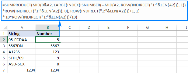
Upon examining the results, however, you may notice one insignificant drawback - if the source string does not contain a number, the formula returns zero, as in row 6 in the screenshot above. To fix this, you can wrap the formula in the IF statement, the logical test of which checks if the source string contains any number. If it does, the formula extracts the number, otherwise returns an empty string:
=IF(SUM(LEN(A2)-LEN(SUBSTITUTE(A2, {"0","1","2","3","4","5","6","7","8","9"}, "")))>0, SUMPRODUCT(MID(0&A2, LARGE(INDEX(ISNUMBER(--MID(A2,ROW(INDIRECT("$1:$"&LEN(A2))),1))* ROW(INDIRECT("$1:$"&LEN(A2))),0), ROW(INDIRECT("$1:$"&LEN(A2))))+1,1) * 10^ROW(INDIRECT("$1:$"&LEN(A2)))/10),"")
As shown in the screenshot below, the improved formula works beautifully (kudos to Alex, our Excel guru, for this improvement):
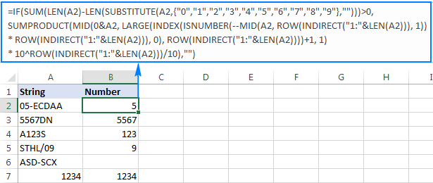
Unlike in all previous examples, the result of this formula is number. To make sure of this, just notice the right-aligned values in column B and truncated leading zeros.
Tip. In Excel 365 - Excel 2019, there is a much simpler solution with the help of the TEXTJOIN function. Please see How to remove text and keep numbers.
Extract number from text string with Ultimate Suite
As you have just seen, there is no trivial Excel formula to pull number from a text string. If you have difficulties with understanding the formulas or tweaking them for your data sets, you may like this simple way to get number from string in Excel.
With our Ultimate Suite added to your Excel ribbon, this is how you can quickly retrieve number from any alphanumeric string:
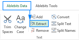
- Go to the Ablebits Data tab > Text group, and click Extract:
- Select all cells with the source strings.
- On the Extract tool's pane, select the Extract numbers radio button.
- Depending on whether you want the results to be formulas or values, select the Insert as formula box or leave it unselected (default).
My advice is to select this box if you want the extracted numbers to update automatically as soon as any changes are made to the source strings. If you want the results to be independent on the original strings (e.g. in case you plan to remove the source data at a later point), then do not select this box.
- Click the Insert Results button. Done!
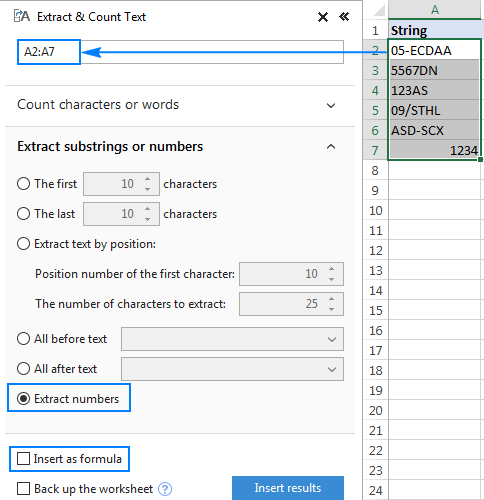
Like in the previous example, the results of the extraction are numbers, meaning you are free to count, sum, average, or perform any other calculations with them.
In this example, we've chosen to insert the results as values, and the add-in did exactly what was asked for:
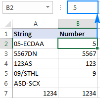
If the Insert as formula checkbox was selected, you'd observe a formula in the formula bar. Curious to know which one? Just download Ultimate Suite's trial and see for yourself :)
Available downloads
Excel Extract Number - sample workbook (.xlsx file)
Ultimate Suite - trial version (.exe file)
 by
by
546 comments
This Formula is working out for me. But is there any solution that I can sumup the values.
Example: 1apple&2orange = 12 (The answer what I am getting as of now but I need to sumup & get "3" as a answer)
Please help me with this.
=IF(SUM(LEN(A2)-LEN(SUBSTITUTE(A2, {"0","1","2","3","4","5","6","7","8","9"}, "")))>0, SUMPRODUCT(MID(0&A2, LARGE(INDEX(ISNUMBER(--MID(A2,ROW(INDIRECT("$1:$"&LEN(A2))),1))* ROW(INDIRECT("$1:$"&LEN(A2))),0), ROW(INDIRECT("$1:$"&LEN(A2))))+1,1) * 10^ROW(INDIRECT("$1:$"&LEN(A2)))/10),"")
Hello!
To extract all numbers from text please use the following formula
=CONCAT(IF(ISNUMBER(--MID(A4,ROW($1:$93),1)),MID(A4,ROW($1:$93),1),""))
Working Fine.
=CONCAT(IF(ISNUMBER(--MID(A4,ROW($1:$93),1)),MID(A4,ROW($1:$93),1),""))
Using the formula
1orrange&2apple = 12 ( Answer getting now)
I need the answer as
1orrange&2apple = 3 ( it suppose to add up the numbers)
Hello!
Replace CONCAT function with SUM:
=SUM((IF(ISNUMBER(--MID(A4,ROW($1:$93),1)),--MID(A4,ROW($1:$93),1),"")))
Hope this is what you need.
500-555-0172
325-555-0137
582-555-0148
1 (21) 500 555-0145
1 (12) 500 555-0117
615-555-0153
926-555-0182
1 (22) 500 555-0140
1 (11) 500 555-0190
961-555-0122
740-555-0182
775-555-0164
Write a formula to extract the numbers, eliminating all the spaces symbols state codes
Hello!
Formula to extract the numbers, eliminating all the spaces symbols and codes —
=CONCAT(IF(ISNUMBER(--MID(REPLACE(A2,1,IFERROR(FIND(")",A2,1),1),""), ROW($1:$93),1)), MID(REPLACE(A2,1,IFERROR(FIND(")",A2,1),1),""), ROW($1:$93),1),""))
I hope my advice will help you solve your task.
Please could you help me with a formula that can extract number from 9 year(s), 11 month(s),
and add a decimal point after years.
Q1- 9 year(s), 11 month(s),
Answer from formula - 9.11
Hello!
The formula below will do the trick for you:
=SUBSTITUTE(TRIM(CONCAT(IF(ISNUMBER(--MID(Q1,ROW($1:$93),1)),MID(Q1,ROW($1:$93),1)," ")))," ",".")
I hope it’ll be helpful.
Dear Expert Users
Please help anybody for get area from 250x350 that is written in one cell
and area should be 87500.
Hello!
Unfortunately, you can only turn text into a formula in Excel using macros. This cannot be done using formulas.
this is the number 15060277631602300000,
i want to separate it like that 1506027763//1602300000
whats the formula for this .please help
Sorry but,
35600aaa bbb/ccc/25*36/450 // Original text.
35600 (O) // The answer I want.
35600aaa bbb(X) // When applying the provided formula.
Can you make an extended formula that meets my requirements?
Sorry but,
I want
25600aaa BBB / 25 * 35 * 46cm
->
25600
I have read well on how to extract numbers from the beginning of a text string.
However, even if there are additional numbers in the middle of the text string, I want to extract only the characters at the beginning in addition to the additional numbers. In other words, if you have a number in the middle of a text string (if the number ends and there is another number after the letter), you want the result to remain unchanged, but the formula provided does not. Is there a possible formula?
Like below
25600aaa bbb/25*35*46cm
Do you have formula, including the decimal point.
Sample: RT-12.5BT, RG5.7T
Because when I use the formula result is
Result: 125, 57
Hello James!
I’m sorry but your task is not entirely clear to me. Could you please describe it in more detail?
Which formula are you using? Explain more precisely what result you want to get? Number with two decimal places?
Hi alexander,
How do i extract number from 113°53'42" to 1135342 ?
Please let me know the formula
Thanks before.
Hello,
Please try the following formula:
=SUBSTITUTE(SUBSTITUTE(SUBSTITUTE(B1,"”",""),"°",""),"’","")
I hope this will help
Thanks for the formula - it works, and it's going to save me a ton of time!
Dear
for example : 25,20,15,25,300,40 is it possible to extract the numbers before "g",
Ali Baba Dark Chocolate 25 gm box 12 pcs
Ali Baba Dark Chocolate 20gm*24 box
Cadbury 5 Star White Chocolate 15gm
Kinder 2 White Chocolate 25 gm*24
ALpella Biscuits W/Marshmallow300gm
Alpella Chocolate 40gm
plz let me know the formula
Hello!
If I understand your task correctly, the following formula should work for you:
=CONCAT(IF(ISNUMBER(--MID(MID(A15, FIND("g",A15,1)-5,5),ROW($1:$93),1)), MID(MID(A15,FIND("g",A15,1)-5,5),ROW($1:$93),1),""))
I hope it’ll be helpful.
hi there,
how do i extract any number before a decimal point using a formula.
meaning 5569.9008 i only want to extract 5569. the formula has to be across for any types of decimals and combination numbers. thank you for the assistance.
Hello!
For decimal use the INT function
=INT(A1)
What is the combination numbers? Google does not know. Neither do I.
I am wondering if this formula can be applied for address street number extraction, wherein the address line you have multiple numbers. For example:
"Rua Hungria, 1240 – Jd. Europa | 1º andar" = 1240 & 1 = 12401
And so, I was hoping for a solution to insert "-" between every occurring number. Thoughts?
This is really great post! Thanks.
Hello Krystian!
I’m sorry but your task is not entirely clear to me. For me to be able to help you better, please describe your task in more detail. Please specify what you were trying to find, what formula you used and what problem or error occurred. Give an example of the source data and the expected result.
It’ll help me understand it better and find a solution for you. Thank you.
Hey Alex!
I am using this formula:
=SUMPRODUCT(MID(0&I25, LARGE(INDEX(ISNUMBER(--MID(I25, ROW(INDIRECT("1:"&LEN(I25))), 1)) * ROW(INDIRECT("1:"&LEN(I25))), 0), ROW(INDIRECT("1:"&LEN(I25))))+1, 1) * 10^ROW(INDIRECT("1:"&LEN(I25)))/10)
And here is the example of raw data:
R LEOPOLDO COUTO DE MAGALHAES JUNIOR, 758 - ANDAR: 15; CONJ: 151;
Using the formula on the above example, I am getting this: 75815151 - concatenated numeric value of all numbers from the string. And, what I am hoping is to add a special character that would show the numbers like so: 758-15-151
In short, on top of extracting the numbers, differentiate multiple numbers by some special character, "-" for example.
Let me know if this is better. Thanks!
Hello Krystian!
You can use a custom format using the TEXT function
=TEXT(A1,"###-##-###")
where A1 is the cell with your formula.
Or use your formula in the TEXT function
=TEXT(SUMPRODUCT(MID(0&I25, LARGE(INDEX(ISNUMBER(--MID(I25, ROW(INDIRECT("1:"&LEN(I25))), 1)) * ROW(INDIRECT("1:"&LEN(I25))), 0), ROW(INDIRECT("1:"&LEN(I25))))+1, 1) * 10^ROW(INDIRECT("1:"&LEN(I25)))/10),"###-##-###")
I hope this will help, otherwise please do not hesitate to contact me anytime.
Hi Alexander, in my case I'd need it more dynamic. Raw data consists of multiple words and there are 2 numbers included. These numbers to be separated by a delimiter.
Is it possible to create this formula without a specific pattern. That it simply extracts the numbers out of a text. no matter how long the text is and how long the numbers are. delimited by a special char such as blank or "-"? Thanks in advance for your help
Example:
client has ordered 500 pieces and wants to have 500 eur in return.
desired result in cell with formula: 500-500
client has exerciesed 500 and wants 3564656,32 new
desired result in cell with formula: 500-3564656,32
Hi,
If I get you right:
To extract numbers "500-500" from text "client has ordered 500 pieces and wants to have 500 eur in return",
use the formula
=SUBSTITUTE(TRIM(CONCAT(IF(ISNUMBER(--MID(A2,ROW($1:$94),1)), MID(A2,ROW($1:$94),1)," ")))," ","-")
I hope this will help
Dear Alexander, thanks for your help on this. It works awesomly. Just had to perform SHIFT+STRG and ENTER in order to get the curly bracket around:-).Highly appreciated.
Dear Alexander, I just wanted to know how the formula could be adpated in order show the below. So if the first and or second number is with mentioning ofcomma/point.
as with previous forumla it shows as below when comma/point are inside the numbers:
500-008-356456-32
raw data:
client has exerciesed 500,008 and wants 3564656,32 new items
desired result in cell with formula:
500,008-3564656,32
raw data:
client has exercesed 500.008 and wants 3564656.32 new
desired result in cell with formula:
500.008-3564656.32
thanks in advance for your help.
Hello!
You want to extract not only numbers, but also text. Comma and period are text. This cannot be done with a single formula. I was able to do this with Abledits Tools. First I used Convert Text (replace letters with spaces), then Trim Spaces (remove extra spaces) and again Convert Text (replace the space between numbers with a dash).
You can install in a trial mode and check how it works for free
If something is still unclear, please feel free to ask.
You can ask a question on the blog or write to support@ablebits.com, include the link to your blog comment.
Thank you in Sharing your "Learned Wisdom "
We learn Every Moment even after the Physical Invisibility of ourselves.
What is the Purpose of Learning if we choose not to share.
Educate a Man" and Thou will Feed the Nations of the World.
Blessings to You
Dear Alexander,
thanks for your hint. Issue is, that on my machine at work I am not allowed to install anything due administrator.
So I hasd to replace the dots and commas by nothing. Then your formula worked well!!
Thanks for your hint with your tool. Wil use it at home:-).
very helpful but please make practice sample files available.
Hi!
You can find the practice sample workbook at the end of this tutorial under "Available downloads".
I want o extract text from number like:
1. 100Rte02T------RTet
how can i do that by using formula
Hello Learner!
To extract all letters from text, use the formula
=SUBSTITUTE((CONCAT(IF(NOT(ISNUMBER( --MID(A1,ROW($1:$93),1))), MID(A1,ROW($1:$93),1),"")))," ","")
Hope this is what you need.
This formula is working but the output is in form of exponential format. I am trying to remove GL code only, but it does not seem to be working.
Here is the example:
Resident Care:69000 · Wellness:69800 · Salaries and Wages:69890 · Payroll Taxes:69891 · FICA
Resident Care:69000 · Wellness:69800 · Salaries and Wages:69890 · Payroll Taxes:69895 · FUTA
Resident Care:69000 · Wellness:69800 · Salaries and Wages:69890 · Payroll Taxes:69897 · MI-UIA
Hello!
I’m sorry but your task is not entirely clear to me.
For me to be able to help you better, please describe your task in more detail. Please let me know in more detail what you were trying to find, what formula you used and what problem or error occurred. It’ll help me understand it better and find a solution for you. Thank you.
Hi Team,
-6.135474.10.00.100012-AziziDevelopments-WO-1-73944857464-CONTR0067799835-Inet
I want to extract only this portion "6.135474.10.00.100012" and some thing like that number from rest of data of 3000. Can anyone help me please with the formula.
Hello Mayank!
If I understand your task correctly, the following formula should work for you
=LEFT(A1,SEARCH("-",A9,2)-1)
I hope this will help, otherwise please do not hesitate to contact me anytime.
Many Many Thanks Alexander. Will try to implement with this new formula.
hi,
Eg: One column 20Pcs Disposable Filter 3 Ply mask and another column 20
how to find the same number exist in that string is correct?
I have tried SEARCH option but is show only position. i want the exact number found in both the column is right/wrong?
Hello!
It is not clear what result you want to get. But maybe this formula is right for you.
=IF(SEARCH(B1,A1,1)>0,"Right","Wrong")
Hope this is what you need.
thank you so much..
THANK YOU SO MUCH THIS SAVED MY LIFE
-6.135474.10.00.100012-AziziDevelopments-WO-1-73944857464-CONTR0067799835-Inet
I want to extract only this portion "6.135474.10.00.100012" and some thing like that number from rest of data of 3000. Can anyone help me please with the formula.
Hi All,
Can you please help me extract this six digit number.
clg:ramanlal/chennai/012345/April
hello Nitin!
To extract a 6-digit number from a mext, use the formula
=MID(A1,MATCH(0, --ISERROR(-MID(A1,ROW($1:$99),1)),),6)
I hope it’ll be helpful.
what is the appropirate formula to find mid value (i.e. 602969) of FP:ADBL5-602969-2830 starting from "FP" among the spread sheet.
Hello!
If I understand your task correctly, please try the following formula:
=MID(A1,FIND("-",A1,1)+1, FIND("-",REPLACE(A1, FIND("-",A1,1),1,""),1)+1 -FIND("-",A1,1)-1)
I hope this will help, otherwise please do not hesitate to contact me anytime.
B264 80 0172760 STAINLESS STEEL HEX HEAD BOLT ASSEMBLY, 1/2" X
What if I'm needing to pull only a seven digit number out of a string of text. I only need the 0172760 from the text. The problem I'm having is that the position of this seven digit number is not consistent from cell to cell and the previously mentioned formulas don't apply because they pull all digits, not just ones with a certain length.
how can i extract set of 6 number form the below string
"LBS 28 Marg, Bhandup West, Mumbai 400078, Maharashtra"
Hello Vinay!
To extract all numbers from text, use the formula
=CONCAT(IF(ISNUMBER( --MID(A1,ROW($1:$93),1)), MID(A1,ROW($1:$93),1),""))
I hope it’ll be helpful.
Hi, could someone please help?
trying to extract the size from the following:
KIERRASTONE ASH TEXTURED ZKI2655A 300 X 600 X 9MM
(300 X 600 X 9MM)
i dont want the numebrs with the text (zki2655a) only the 300 X 600 X 9MM
thanks look forward to your reply :)
Hello Peter!
If I understand your task correctly, the following formula should work for you:
=MID(A1,FIND("(",A1,1)+1,LEN(A1)-FIND("(",A1,1)-1)
I hope this will help, otherwise please do not hesitate to contact me anytime.
Hi How do I find the MAX numerical value of the alphanumeric string? for example:
X-0100
B-0213
F-0505
Z-0111
to show that F-0505 is the high value in the column
Hello Kevin!
If I understand your task correctly, the following formula should work for you
=INDEX(A1:A5,MATCH("*"&LARGE( --RIGHT(A1:A5,LEN(A1:A5) - FIND("-",A1:A5)),1),A1:A5,0))
If there is anything else I can help you with, please let me know.
What would be the number if the invoice number has alphanumeric characters in the middle.
Example:
09187GH1234
Hello, what formula can I use to pull and separate the last four sets of numbers in the following string?
"CJFRO20190047 000 004 03/14/19 1906 JP MORGA JPMC 1st Qtr 0.00 0.00 0.00 -12.63"
I used the first formula from above but it doesn't give me all the values.
Any advice will be greatly appreciated.
Thanks for this great solution. The formula given above ("How to get number from any position in a string")-> is work fine.
What is a good formula to use in order to see numbers that are alike in any order? For example
457. 885
886. 275
573. 547
Below formula working fine but some number have percent sign between the text,i want extract number with percent sign which have % Sign as well.
=IF(SUM(LEN(A2)-LEN(SUBSTITUTE(A2, {"0","1","2","3","4","5","6","7","8","9"}, "")))>0, SUMPRODUCT(MID(0&A2, LARGE(INDEX(ISNUMBER(--MID(A2,ROW(INDIRECT("$1:$"&LEN(A2))),1))* ROW(INDIRECT("$1:$"&LEN(A2))),0), ROW(INDIRECT("$1:$"&LEN(A2))))+1,1) * 10^ROW(INDIRECT("$1:$"&LEN(A2)))/10),"")
hi i have a cell from vendor quotes that i receive. this is how i name the vendor quote.
Lighting Expression 11-20-19 ($132,833)
Vendor name - date provided - dollar amount
i want to extract only the dollar amount which can vary up to 2 million.
How can add the numbers of this following examples, without sorting it fisrt
CIVUS0.35B
CIVUS1W
IA-CIVUS0.13W
TAVUS0.35SB
AVSSF2W/B
AVS3W/B
The article was such Helpful that I got rid of a work that could have required me to dedicate lots of minutes. Thank you all.
Thanks for the formulas (But I had trouble get them working. Here is why)
In some countries, Sweden among them, the "," character is a decimal delimiter. There for "SEARCH({0,1,2,3,4,5,6,7,8,9},A2)" results in an error. So for us we have to use another character in the syntax, ";". So here is what worked for me:
SEARCH({0;1;2;3;4;5;6;7;8;9},A2)
Hope above saves some time for others!
if character is more then 10 and less then 1000 which formula use
=SUM(MID(0&A3,LARGE(ISNUMBER(--MID(A3,ROW(INDIRECT("1:"&LEN(A3)))*ROW(INDIRECT("1:"&LEN(A3))),1)),ROW(INDIRECT("1:"&LEN(A3))))+1,1)*10^(ROW(INDIRECT("1:"&LEN(A3)))-1))
not getting any result if help if there is any error
This formula does not give the decimal values i.e 5.25, 7.3 and more. Kindly help me out on this.
Formula ,
IF(SUM(LEN(A2)-LEN(SUBSTITUTE(A2, {"0","1","2","3","4","5","6","7","8","9"}, "")))>0, SUMPRODUCT(MID(0&A2, LARGE(INDEX(ISNUMBER(--MID(A2,ROW(INDIRECT("$1:$"&LEN(A2))),1))* ROW(INDIRECT("$1:$"&LEN(A2))),0), ROW(INDIRECT("$1:$"&LEN(A2))))+1,1) * 10^ROW(INDIRECT("$1:$"&LEN(A2)))/10),"")
=LOOKUP(9.9E+307,--LEFT(MID(A2,MIN(FIND({1,2,3,4,5,6,7,8,9,0}, $A2&"1023456789")),999),ROW(INDIRECT("1:999"))))
While this was very very helpful, I am facing a new kind of problem.
Job Id - #2416387528594195 is getting converted to '2416387528594190, excel is rounding off the last two digits and replacing with 0. Concat with an apostrophe also didn't help. I applied formula: =CONCAT("'",SUMPRODUCT(MID(0&B2,LARGE(INDEX(ISNUMBER(--MID(B2,ROW(INDIRECT("1:"&LEN(B2))),1))*ROW(INDIRECT("1:"&LEN(B2))),0),ROW(INDIRECT("1:"&LEN(B2))))+1,1)*10^ROW(INDIRECT("1:"&LEN(B2)))/10))
Hey,
Svetlana Cheusheva
Thank you so much for the tutorial. It is very nice of you. It was very helpful to me.
This formula is exactly what I was looking for... and it works perfectly. Thank you so much! ;-)
=IF(SUM(LEN(A2)-LEN(SUBSTITUTE(A2, {"0","1","2","3","4","5","6","7","8","9"}, "")))>0, SUMPRODUCT(MID(0&A2, LARGE(INDEX(ISNUMBER(--MID(A2,ROW(INDIRECT("$1:$"&LEN(A2))),1))* ROW(INDIRECT("$1:$"&LEN(A2))),0), ROW(INDIRECT("$1:$"&LEN(A2))))+1,1) * 10^ROW(INDIRECT("$1:$"&LEN(A2)))/10),"")
Not sure how to extract check no’s. From a text string having more that one set of numbers - see example below:
Brad James Company - Check - 23897 / invoice # 456755 issued Sept 1
Any suggestions are greatly appreciated - the line above is a sample of the excel items and after the check number shown there a number of invoice numbers in the text string.
Thanks , Fred
If this is the data :
My Assumption is that all your data has "/" after the check number.
First :
Find the nth place of that "/" in that string using this formula :
=+FIND("/",D2)
Brad James Company - Check - 23897 / invoice # 456755 issued Sept 1
Output = 36
then,
use this formula =+MID(D2,C2-7,7)
here D2 is the input data which you have & C2 refers to the output of find formula i.e)36
then the output will be "23987".
Hope this helps! :)
The formula, of middle search doesnt fetch n give decimal place like 18.625
Client Name
LALITA
GEETA DEVI NAYAK
MEHARUN NISHA
DIPA MANOJ
PREETI SINGHAL
meena devi swami
RAJIYA BEGAM
SHEHIDE
TARAWATI
BHATERI DEVI
sheela devi
JANKI DEVI
SUNITA
ALKA KANWAR
JAITUN
POOJA DEBI
CHHOTI DEVI
VIMLA DEVI
manju devi tak
MANJU
MUNNI DEVI
GEETA DEVI
TULSI DEVI
AILARAKHI
MUMTAJ BIBI
How to Find MID name if mid name more than 3 Character
=IF((LEN(A2)-LEN(SUBSTITUTE(A2," ","")))>1,MID(A2,FIND(" ",A2,1)+1,SUM(FIND(" ",A2,FIND(" ",A2,1)+1),(FIND(" ",A2,1)+1)*-1)),"")
Ram mobile no-9925923457. Resides In Noida 119961
Can You suggest How To find Phn no. From Above Text
According to your para, find the number first, once you get all the numeric, then take the left 10 digits, using the left formula.
This is a great post.
thank you so much for your effort here. I wish my company wasn't so tight in the pockets so I could get all those add-ins
Hi,
This is very helpful.
One thing, the SUBSTITUTE(A2,{"0","1","2","3","4","5","6","7","8","9"},"") doesn't seem to be working for me. It is not replacing the characters with empty string.
Data in cell A2: 25R
Expected: R
I meant, how do I get the last method (extract from anywhere) to preserve leading 0's? Thanks.
This was immensely helpful, thanks. How do I get it to preserve any leading zeroes?
Hey,
Svetlana Cheusheva
Please tell me how I can make a live input cell that is
"Underlying Index: NIFTY 11907.30 As on Jul 03, 2019 10:05:20 IST" in B1 CELL
to another cell say in C1 11907.30 and time in C2 10:50:20 to another cell.
or at least I can print C1 that would be also sufficient.
mainly viewed all the comment but not able to figure the amount