The tutorial shows how to calculate IRR of a project in Excel with formulas and the Goal Seek feature. You will also learn how to create an internal rate of return template to do all IRR calculations automatically.
When you know the internal rate of return of a proposed investment, you may think you have all you need to evaluate it - the bigger the IRR the better. In practice, it's not that simple. Microsoft Excel provides three different functions to find the internal rate of return, and truly understanding what you are actually calculating with IRR will be very helpful.
What is IRR?
The internal rate of return (IRR) is a commonly used metric to estimate the profitability of a potential investment. Sometimes, it is also referred to as discounted cash flow rate of return or economic rate of return.
Technically, IRR is the discount rate that makes the net present value of all cash flows (both inflows and outflows) from a certain investment equal to zero.
The term "internal" indicates that IRR takes into account only internal factors; external factors such as inflation, the cost of capital and various financial risks are excluded from calculation.
What does the IRR reveal?
In capital budgeting, IRR is widely used to evaluate the profitability of a prospective investment and rank multiple projects. The general principle is as simple as this: the higher the internal rate of return, the more attractive the project is.
When estimating a single project, finance analysts typically compare the IRR to a company's weighted average cost of capital or hurdle rate, which is the minimum rate of return on an investment that the company can accept. In a hypothetical situation, when IRR is the only criterion for making a decision, a project is considered a good investment if its IRR is greater than the hurdle rate. If the IRR is lower than the cost of capital, the project should be rejected. In practice, there are a lot of other factors that influence the decision such as the net present value (NPV), payback period, absolute return value, etc.
IRR limitations
Though IRR is a very popular method for assessing capital projects, it does have a number of inherent flaws that may lead to suboptimal decisions. The main problems with IRR are:
- Relative measure. IRR considers percentage but not the absolute value, as the result, it can favor a project with a high rate of return but a very small dollar value. In practice, companies may prefer a large project with a lower IRR over a small one with a higher IRR. In this respect, NPV is a better metric because it considers an actual amount gained or lost by undertaking a project.
- The same reinvestment rate. IRR assumes that all cash flows generated by a project are reinvested at the rate equal to the IRR itself, which is a very unrealistic scenario. This problem is solved by MIRR that allows specifying different finance and reinvest rates.
- Multiple results. For projects with alternating positive and negative cash flows, more than one IRR can be found. The issue is also resolved in MIRR, which is designed to produce only one rate.
Despite these deficiencies, IRR continues to be an important measure of capital budgeting and, at the very least, you should cast a skeptical look at it before making an investment decision.
IRR calculation in Excel
As the internal rate of return is the discount rate at which the net present value of a given series of cash flows is equal to zero, the IRR calculation is based on the traditional NPV formula:
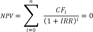
If you are not very familiar with the summation notation, the extended form of the IRR formula may be easier to understand:
![]()
Where:
- CF0 - the initial investment (represented by a negative number)
- CF1, CF2 … CFn - cash flows
- i - the period number
- n - periods total
- IRR - internal rate of return
The nature of the formula is such that there is no analytical way to calculate IRR. We have to use the "guess and check" approach to find it. To better understand the concept of the internal rate of return, let's perform an IRR calculation on a very simple example.
Example: You invest $1000 now and get back $500 and $660 in the next 2 years. What discount rate makes the Net Present Value zero?
As our first guess, let's try 8% rate:
- Now: PV = -$1,000
- Year 1: PV = $500 / (1+0.08)1 = $462.96
- Year 2: PV = $660 / (1+0.08)2 = $565.84
Adding those up, we get the NPV equal to $28.81:
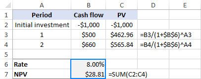
Oh, not even close to 0. Maybe a better guess, say 10%, can change things?
- Now: PV = -$1,000
- Year 1: PV = $500 / (1+0.1)1 = $454.55
- Year 2: PV = $660 / (1+0.1)2 = $545.45
- NPV: -1000 + $454.55 + $545.45 = $0.00
That's it! At 10% discount rate, the NPV is exactly 0. So, the IRR for this investment is 10%:
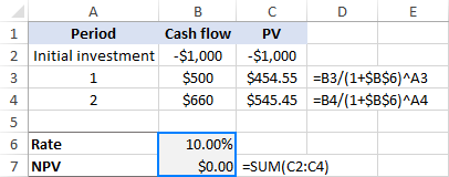
That's how you calculate the internal rate of return manually. Microsoft Excel, other software programs and various online IRR calculators also rely on this trial and error method. But unlike humans, computers can do multiple iterations very quickly.
How to calculate IRR in Excel with formulas
Microsoft Excel provides 3 functions for finding the internal rate of return:
- IRR - the most commonly used function to calculate the internal rate of return for a series of cash flows that occur at regular intervals.
- XIRR – finds IRR for a series of cash flows that occur at irregular intervals. Because it takes into consideration the exact dates of payments, this function provides a better calculation accuracy.
- MIRR – returns the modified internal rate of return, which is a variant of IRR that considers both the cost of borrowing and compounded interest received on the reinvestment of positive cash flows.
Below you will find the examples of all these functions. For the sake of consistency, we will be using the same data set in all the formulas.
IRR formula to calculate internal rate of return
Suppose you are considering a 5-year investment with the cash flows in B2:B7. To work out the IRR, use this simple formula:
=IRR(B2:B7)
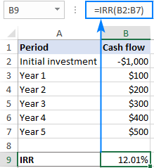
Note. For the IRR formula to work correctly, please make sure that your cash flows have at least one negative (outflow) and one positive value (inflow), and all the values are listed on chronological order.
For more information, please see the Excel IRR function.
XIRR formula to find IRR for irregular cash flows
In case of cash flows with unequal timing, using the IRR function can be risky, as it assumes that all payments occur at the end of a period and all time periods are equal. In this case, XIRR would be a wiser choice.
With the cash flows in B2:B7 and their dates in C2:C7, the formula would go as follows:
=XIRR(B2:B7,C2:C7)
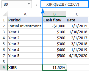
Notes:
- Though the XIRR function does not necessarily require dates in chronological order, the date of the first cash flow (initial investment) should be first in the array.
- The dates must be provided as valid Excel dates; supplying dates in text format puts Excel at risk of misinterpreting them.
- The Excel XIRR function uses a different formula to arrive at a result. The XIRR formula discounts subsequent payments based on a 365-day year, as the result, XIRR always returns an annualized internal rate of return.
For more details, please see the Excel XIRR function.
MIRR formula to work out the modified IRR
To handle a more realistic situation when the project funds are reinvested at a rate closer to a company's cost of capital, you can compute the modified internal rate of return by using a MIRR formula:
=MIRR(B2:B7,E1,E2)
Where B2:B7 are cash flows, E1 is the finance rate (the cost of borrowing the money) and E2 is the reinvest rate (the interest received on the reinvestment of earnings).
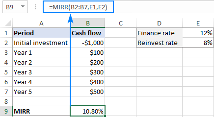
Note. Because the Excel MIRR function computes compound interest on profits, its result may be substantially different from those of the IRR and XIRR functions.
IRR, XIRR and MIRR - which is better?
I believe no one can give a generic answer to this question because the theoretical basis, advantages and drawbacks of all three methods are still disputed among finance academics. Perhaps, the best approach would be to do all three calculations and compare the results:
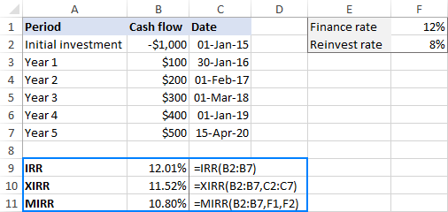
Generally, it is considered that:
- XIRR provides better calculation accuracy than IRR because it takes into consideration the exact dates of cash flows.
- IRR often gives an unduly optimistic assessment of the project's profitability, while MIRR gives a more realistic picture.
IRR calculator - Excel template
If you need to do IRR calculation in Excel on a regular basis, setting up an internal rate of return template can make your life a lot easier.
Our calculator will include all three formulas (IRR, XIRR, and MIRR) so that you won't have to worry which result is more valid but could consider them all.
- Input the cash flows and dates in two columns (A and B in our case).
- Enter the finance rate and reinvest rate in 2 separate cells. Optionally, name these sells Finance_rate and Reinvest_rate, respectively.
- Create two dynamic defined ranges, named Cash_flows and Dates.
Assuming your worksheet is named Sheet1, the first cash flow (initial investment) is in cell A2, and the date of the first cash flow is in cell B2, make the named ranges based on these formulas:
Cash_flows:
=OFFSET(Sheet1!$A$2,0,0,COUNT(Sheet1!$A:$A),1)Dates:
=OFFSET(Sheet1!$B$2,0,0,COUNT(Sheet1!$B:$B),1)The detailed steps can be found in How to create a dynamic named range in Excel.
- Use the names you have just created as arguments of the following formulas. Please note that the formulas can be entered in any column other than A and B, which are reserved exclusively for cash flows and dates, respectively.
=IRR(Cash_flows)=XIRR(Cash_flows, Dates)=MIRR(Cash_flows, Finance_rate, Reinvest_rate)
Done! You can now input any number of cash flows in column A, and your dynamic internal rate of return formulas will recalculate accordingly:

As a precaution against careless users who may forget to fill all the required input cells, you can wrap your formulas in the IFERROR function to prevent errors:
=IFERROR(IRR(Cash_flows), "")
=IFERROR(XIRR(Cash_flows, Dates), "")
=IFERROR(MIRR(Cash_flows, Finance_rate, Reinvest_rate), "")
Please keep in mind that if the Finance_rate and/or Reinvest_rate cells are blank, the Excel MIRR function assumes they are equal to zero.
How to do IRR in Excel with Goal Seek
The Excel IRR function only performs 20 iterations to arrive at a rate and XIRR performs 100 iterations. If after that many iterations a result accurate within 0.00001% is not found, a #NUM! error is returned.
If you are looking for more accuracy for your IRR calculation, you can force Excel to do over 32,000 iterations by using the Goal Seek feature, which is part of What-If Analysis.
The idea is to get Goal Seek to find a percentage rate that makes the NPV equal to 0. Here's how:
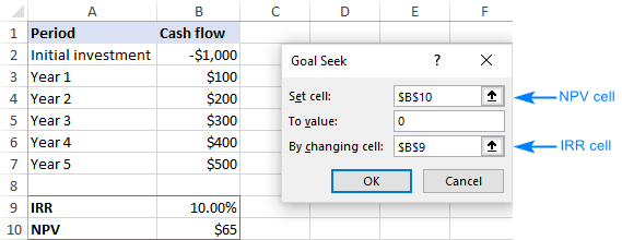
- Set up the source data in this way:
- Enter the cash flows in a column (B2:B7 in this example).
- Put the expected IRR in some cell (B9). The value that you enter does not actually matter, you just need to "feed" something to the NPV formula, so just put any percentage that comes to mind, say 10%.
- Enter the following NPV formula in another cell (B10):
=NPV(B9,B3:B7)+B2
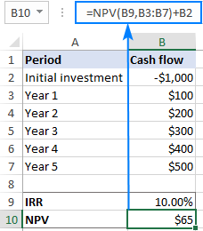
- On the Data tab, in the Forecast group, click What if Analysis > Goal Seek…
- In the Goal Seek dialog box, define the cells and values to test:
- Set cell - the reference to the NPV cell (B10).
- To value – type 0, which is the desired value for the Set cell.
- By changing cell - the reference to the IRR cell (B9).
When done, click OK.
- The Goal Seek Status dialog box will appear and let you know if a solution has been found. If successful, the value in the IRR cell will be replaced with a new one that makes NPV zero.
Click OK to accept the new value or Cancel to get back the original one.

In a similar manner, you can use the Goal Seek feature to find XIRR. The only difference is that you will need to use the XNPV formula instead of NPV.
Note. The IRR value found with Goal Seek is static, it does not recalculate dynamically as formulas do. After each change in the original data, you will have to repeat the above steps to get a new IRR.
That's how to do IRR calculation in Excel. To have a closer look at the formulas discussed in this tutorial, you are welcome to download our sample workbook below. I thank you for reading and hope to see you on our blog next week!
Practice workbook for download
Excel IRR Calculator - examples (.xlsx file)
 by
by
2 comments
Thank you!!!
Dear Svetlana,
Thank you for such enlightening write-ups. Much appreciated.
I'm trying to find out the real-world realized returns of my ETF investments. It is always represented in Annualized return, which is not the "actual" return that I might be getting due to market volatility. To me, I believe, IRR is the actual realized return. Correct me if I'm wrong.
How do I make an IRR calculation sheet for daily cash flow, because I randomly buy funds at multiple intervals.
Kindly advise.