This tutorial will teach you a few quick ways to insert superscript and subscript in Excel, both for text values and numbers.
Microsoft Office users sometimes wonder why a particular feature is present in one Office application and absent in another. So is the case with superscript and subscript formats - available on the Word ribbon, they are nowhere to be found in Excel. Please remember, Microsoft Word is all about text and Excel is about numbers, it can't do all Word tricks. However, it does have a lot of tricks of its own.
What is superscript and subscript in Excel?
Superscript is a small letter or number typed above the baseline. If there is any preceding text in a cell, superscript is attached to the top of the regular sized characters.
For example, you can use superscript to write square units like m2 or inch2, ordinal numbers such as 1st, 2nd, or 3rd, or exponents in math such as 23 or 52.
Subscript is a small character or string that sits below the line of text.
In math, it is often used to write number bases like 648 or chemical formulas such as H2O or NH3.
How to do superscript and subscript for text values
Most Excel formatting can be applied to any data type in the same way. Superscript and subscript are a different story. The methods described in this section work only for text values, but not for numbers. Why? I believe only the Microsoft team know the exact reason :) Possibly because this would convert numbers to strings and they want to prevent you from accidentally mangling your data.
Apply superscript or subscript format
Every time you want to format text in Excel, open the Format Cells dialog box. It allows you to quickly apply the superscript, subscript, and strikethrough effect or whatever formatting you want.
In case of superscript and subscript, there is one hurdle. You can't just apply the format normally to the entire cell because this would move all the text above or below the baseline, which is almost certainly not what you want.
Here are the steps to insert subscript or superscript correctly:
- Select the text you'd like to format. For this, double click a cell and select the text using the mouse. Or you can go the old-fashioned way - click the cell and press F2 to enter edit mode.
- Open the Format Cells dialog by pressing Ctrl + 1 or right-click the selection and choose Format Cells… from the context menu.

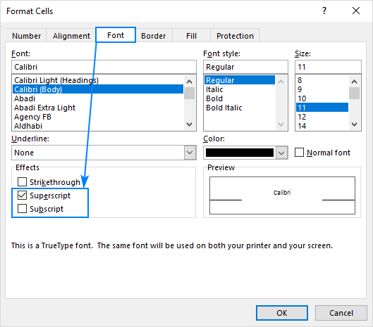
- In the Format Cells dialog box, go to the Font tab, and select Superscript or Subscript under Effects.

- Click OK to save the change and close the dialog.
Done! The selected text will be subscripted or superscripted depending on which option you've ticked off.
Note. Like any other formatting in Excel, it changes only visual representation of the value in a cell. The formula bar will display the original value without any indication of the applied superscript or subscript format.

Keyboard shortcuts for superscript and subscript in Excel
Although there is no shortcut in its pure sense to add subscript or superscript in Excel, this can be done with a couple of key combinations.
Excel superscript shortcut
Ctrl + 1, then Alt + E, and then Enter

Excel subscript shortcut
Ctrl + 1, then Alt + B, and then Enter

Please pay attention that the keys should not be pressed simultaneously, each key combination should be pressed and released in turn:
- Select one or more characters you want to format.
- Press Ctrl + 1 to open the Format Cells dialog box.
- Then press either Alt + E to select the Superscript option or Alt + B to select Subscript.
- Hit the Enter key to apply the formatting and close the dialog.
Add Superscript and Subscript icons to Quick Access Toolbar
In Excel 2016 and higher, you can also add the Subscript and Superscript buttons to their Quick Access Toolbar (QAT). Here are the steps for this one-time setup:
- Click the down arrow next to the QAT in the upper left corner of the Excel window, and choose More Commands… from the pop-up menu.

- Under Choose commands from, select Commands Not in the Ribbon, scroll down, select Subscript in the list of commands, and click the Add button.
- In the same way, add the Superscript button.
- With both buttons added to the list of commands on the right pane, click OK to save the changes.

And now, you can simply select the text to be subscripted or superscripted in a cell or in the formula bar, and click the corresponding icon on the Quick Access Toolbar to apply the format:

Moreover, a special keyboard shortcut is assigned to each Quick Access Toolbar button enabling you to subscript and superscript in Excel 2016 with a single key stroke! The key combinations vary depending on how many buttons your QAT accommodates.
To find out the superscript and subscript shortcuts on your computer, hold the Alt key and look at the Quick Access Toolbar. For me, they are as follows:
- Subscript shortcut: Alt + 4
- Superscript shortcut: Alt + 5

Add Subscript and Superscript buttons to Excel ribbon
If you'd rather not clutter your Quick Access Toolbar with too many icons, you can add the Superscript and Subscript buttons to your Excel ribbon.
Because custom buttons can only be added to custom groups, you will have to create one. Here's how:
- Right-click anywhere on the ribbon and select Customize the Ribbon… from the pop-up menu. This opens the Excel Options dialog box.
- In the right part of the dialog box, under Customize the Ribbon, select the desired tab, say Home, and click the New Group button.
- Click the Rename button to give the newly added group a name you like, e.g. My Formats. At this point, you will have the following result:

- In the left-hand drop-down list, under Choose commands from, select Commands Not in the Ribbon, then choose Superscript in the list of commands, and click Add.
- Next, select Subscript in the list of commands and click the Add button again.

- Click OK to save the changes and close the dialog box.
Now, you can subscript and superscript in Excel by clicking the corresponding button on the ribbon:

How to remove subscript and superscript formatting in Excel
Depending on whether you want to remove all or particular subscripts/superscripts in a cell, select the entire cell or only the subscripted/superscripted text, and do the following:
- Press Ctrl + 1 to open the Format Cells… dialog box.
- On the Font tab, clear the Superscript or Subscript checkbox.
- Click OK.
The subscript and superscript formats can also be deleted by pressing the respective keyboard shortcut or clicking the corresponding button on the ribbon and QAT if such buttons are added in your Excel.
Apply superscript and subscript format to numbers
Below, you will find a few techniques to do superscript and subscript for numeric values. Please keep in mind that some of the methods convert numbers to strings, while others change only a visual display of the value in a cell. To see the actual value behind a superscript, look at the formula bar. Also, please be sure to carefully read the limitations of each method before using it in your worksheets.
How to write subscript and superscript in Excel
To be able to type subscript and superscript in Excel, insert an equation in your worksheet. Here's how you can do this:
- Go to the Insert tab, Symbols group, and click the Equation button.

- This will take you to the Design tab, where you click the Script button in the Structures group, and select the desired format, for example Superscript.

- Click the squares, type your values, and you are done!

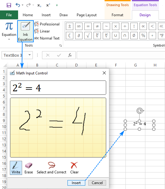
Alternatively, you can click the Ink Equation button and write your math using the mouse. If Excel understands your handwriting, it will show the preview correctly. Clicking the Insert button will insert your input in a worksheet.

Caveats: This method inserts your math as an Excel object, not cell value. You can move, resize and rotate your equations by using the handles, but you cannot reference them in formulas.
Excel superscript shortcuts for numbers
Microsoft Excel provides an easy way to insert superscripted numbers in cells, as long as they are 1, 2, or 3. Simply type the following numbers on the numeric keypad while holding down the Alt key:
| Superscript | Shortcut |
| 1 | Alt+0185 |
| 2 | Alt+0178 |
| 3 | Alt+0179 |
By using these shortcuts, you can type superscripts in empty cells and attach them to existing numbers:

Caveats:
- These shortcuts work for Calibri and Arial If you are using some other font, the character codes may be different.
- The numbers with superscripts are turned into numeric strings, meaning you won't be able to perform any calculations with them.
How to make superscript in Excel with a formula
Another quick way to do superscript in Excel is by using the CHAR function with the corresponding code.
Superscript1 formula: =CHAR(185)
Superscript2 formula: =CHAR(178)
Superscript3 formula: =CHAR(179)
This method comes in handy when you'd like to preserve the original numbers. In this case, you concatenate the CHAR function with the original number and enter the formula in the next column.
For example, that's how you can add superscript two to the number in A2:
=A2&CHAR(178)

Caveat: As with the previous method, the formula output is a string, not number. Please notice the left-aligned values in column B and right-aligned numbers in column A in the screenshot above.
How to superscript and subscript in Excel with custom format
If you'd like to add superscript to a range of numbers, a faster way would be creating a custom format. Here's how:
- Select all the cells to be formatted.
- Press Ctrl + 1 to open the Format Cells… dialog.
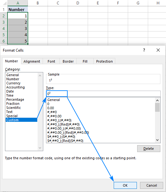
- On the Number tab, under Category, select Custom.
- In the Type box, enter 0, which is the digit placeholder, then hold the Alt key as you type the corresponding superscript code.
For example, to create a custom number format for superscript 3, type 0, press the Alt key, type 0179 on the numeric keypad, then release Alt.
- Click OK.

The superscripted numbers will look similar to this:

To make a custom subscript format or superscript format with numbers other than 1, 2, or 3, copy the needed character from here. For example, to insert superscript 5, set up a custom format with this code: 0⁵. To add subscript 3, use this code: 0₃.
To remove superscripts, simply set the cell format back to General.
Caveat: Unlike the previous method, Excel custom number format does not change the original value in a cell, it only changes the visual representation of the value. In the above screenshot, you can see 1³ in cell A2, but the formula bar displays 1, meaning the actual value in the cell is 1. If you reference A2 in formulas, its real value (the number 1) will be used in all calculations.
How to do superscript in Excel with VBA
In case you need to quickly add a certain superscript to the entire column of numbers you can automate the creation of a custom number format with VBA.
Here is a simple one-line macro to add Superscript Two to all selected cells.
To add other superscripts, replace Chr(178) with the corresponding character code:
Superscript One: Chr(185)
Superscript Three: Chr(179)
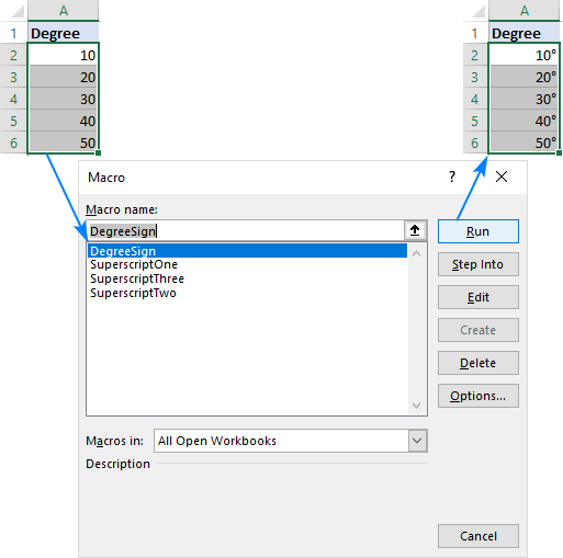
This macro can also be used to attach the degree sign to the numbers in the selected cells. For this, use Chr(176), and your numbers will get formatted in this way:

The step-by-step instructions on how to insert and run VBA code in Excel can be found here. Or, you can download our sample workbook with all superscript macros and open it alongside your own workbook. Then, in your workbook, press Alt + F8, select the desired macro, and click Run.
Super easy way to superscript and subscript in Excel - copy and paste!
Microsoft Excel does not provide shortcuts or character codes to insert superscripted numbers other than 1, 2 or 3. But we know that the impossibility is nothing :) Simply copy the subscripted and superscripted numbers and mathematical symbols from here:
Subscripts: ₀ ₁ ₂ ₃ ₄ ₅ ₆ ₇ ₈ ₉ ₊ ₋ ₌ ₍ ₎
Superscripts: ⁰ ¹ ² ³ ⁴ ⁵ ⁶ ⁷ ⁸ ⁹ ⁺ ⁻ ⁼ ⁽ ⁾
Apart from simplicity, this method has one more advantage - it allows you to add subscripts and superscripts to any cell value, text and numbers!
If you need Unicode subscript and superscript letters and symbols, you can copy them from this Wikipedia article.
That's how to use subscript and superscript formats in Excel. I thank you for reading and hope to see you on our blog next week!
 by
by
15 comments
It is, by all means, a great tutorial. You have done an excellent, user-friendly, professional work.
Thank you very much for your kind words!
Great article very helpful. I would like to have 4 options in a drop down menu that contain a mixture of units, eg cm, cm2, m and m2. Is it possible to have the 2 in the options as superscript??
Thanks
cm
cm2
m
m3
Use these in a values in a sheet and refer this as source for the List to be considered for the drop down.
I.e., source = =$C$23:$C$26
Can you tell how to subscript/superscript in "Google Sheets" ? None of these work there.
Even google docs command "ctrl+, " is not working in sheets.
Hello Alex,
for Google Sheets, you can write in subscript/superscript only with the help of the CHAR function. It uses Unicode as a base.
Here's the link for all characters available in superscripts and subscripts:
https://www.unicode.org/charts/PDF/U2070.pdf
Thanks Darling!
="Dated this the "&TEXT(TODAY(),"dd")&"ᵗʰ"&" day of "&TEXT(TODAY(),"MMMM")&", 2019"
How about 1st and 2nd, can you share with me that fonts?
I leave this here for anyone who struggle with the same problem in the future...
ˢᵗ , ⁿᵈ , ʳᵈ , ᵗʰ
Can you help for superscript 2 - 3 (Ex: m^2, m^3) as well bro?
I tried the ctrl1 for superscript and it worked but the moment I move to the next bar it goes back to the same number without subcript.why is that?
I have this same problem. When I double click on the cell it shows the superscript formatting but if I click out of that cell it goes away.
why i could not use CHAR function to generate superscript? When i input formula =A2&Char(185), it always shows Char(185) as empty or blank.
Tdat:
The character returned is based on the character set used by your computer. Entering A2&CHAR(185) in A3 should add the superscript to the number displayed in A3 to the number displayed in A2.
You can see the character set you are currently using and change to another set in Win 10 by:
Open Control Panel, go to Clock, Language, and Region,select Region. Now the Region wizard opens and the Administrative tab is there. You can see your region and language and add a language if needed.
However, this will change all the characters you use on your computer.