Filtering huge tables helps focus your attention on the most needed information. Today I'd like to discuss with you the ways of adding filters by condition, even applying a few of them to your data at once. I will also explain why the Google Sheets filter is so useful and important when you work within a shared document.
Filter by condition in Google Sheets
Let's start by applying a basic filter to the Google sheet. If you don't know or don't remember how to do that, please check my previous blog post.
When the corresponding icons are there on column headers, click the one that belongs to the column you want to work with and choose Filter by condition. An additional option field will appear, with the word "None" in it.
Click on it, and you'll see the list of all conditions available to filter in Google Sheets. If none of the existing conditions meets your needs, you're free to create your own one by choosing Custom formula is from the list:
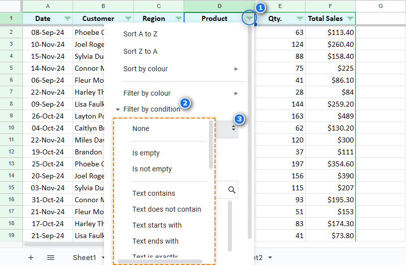
Let's look through them together, shall we?
Is not empty
If cells contain numeric values and/or text strings, logical expressions, or any other data including spaces ( ) or empty strings (""), the rows with such cells will be displayed.
You can get the same result using the following formula when selecting the Custom formula is option:
=ISBLANK(B:B)=FALSE
Is empty
This option is completely opposite to the previous one. Only cells that don't have any contents in them will be displayed. Others will be filtered out by Google Sheets.
You can also use this formula:
=ISBLANK(B:B)=TRUE
Text contains
This option shows rows where cells contain specific characters – numeric and/or textual. It doesn't matter whether they are at the beginning, in the middle, or at the end of a cell.
You can use wildcard characters to find some specific symbols in different positions within a cell. Asterisk (*) is used to substitute any number of characters while a question mark (?) replaces a single symbol:
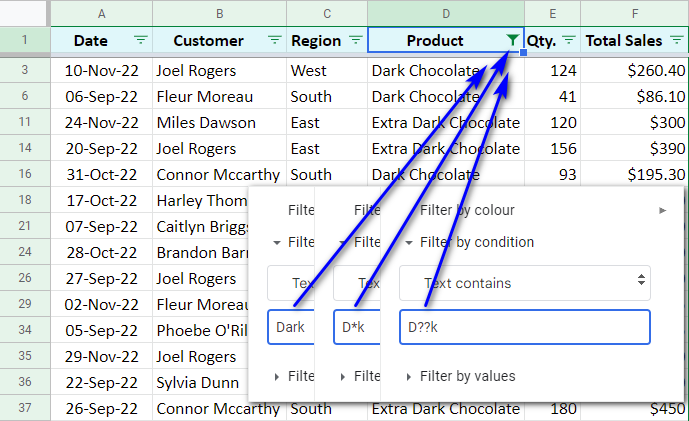
As you can see, you can achieve the same result by entering various wildcard char combos.
The following formula will also help:
=REGEXMATCH(D:D,"Dark")
Text does not contain
I believe you already understand that the conditions here can be the same as in the point above, but the result will be the opposite. The value you enter will be filtered out from the Google Sheets view.
As for the custom formula, it can look as follows:
=REGEXMATCH(D:D,"Dark")=FALSE
Text starts with
For this condition, enter the first character(s) (one or more) of the value of interest.
Note. Wildcard characters don't work here.
Text ends with
Alternatively, enter the last characters of the entries you need to display.
Note. Wildcard characters also can't be used here.
Text is exactly
Here you need to enter exactly what you want to see, whether it's a number or text. Milk Chocolate, for example. Entries that contain something other than that won't be displayed. Thus, you can't use wildcard characters here.
Note. Please keep in mind that the text case matters for this condition.
If you want to use a formula to search for all records that contain "Milk Chocolate" only, enter the following:
=D:D="Milk Chocolate"
Date is, Date is before, Date is after
These Google Sheets filters allow using dates as conditions. As a result, you'll see the rows that contain an exact date or the date before/after the exact date.
Default options are today, tomorrow, yesterday, in the past week, in the past month, in the past year. You can also enter an exact date:
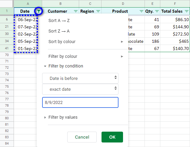
Note. When you enter any date, make sure to type it in your regional settings format rather than its format in the table. You can read more about date and time formats here.
Google Sheets filter for numeric values
You can filter numeric data in Google Sheets by the following conditions: greater than, greater than or equal to, less than, less than or equal to, is equal to, is not equal to, is between, is not between.
The last two conditions require two numbers that indicate starting and ending points of the desired interval.
Tip. You can use cell references as conditions considering that cells you refer to contain numbers.
I want to see the rows where numbers in column E are greater than or equal to the value in G1:
=$G$1
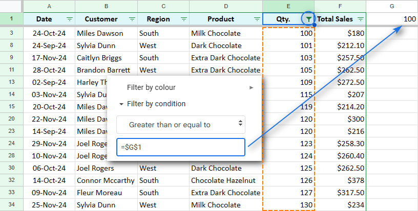
Note. If you change the number you refer to (100 in my case), the displayed range won't update automatically. Click the Filter icon on your Google Sheets column and then OK to update the results manually.
The custom formula can be used for this option as well.
=E:E>$G$1
Custom formulas to filter by condition in Google Sheets
Each of the aforementioned options can be replaced by custom formulas that return the same result.
Yet, formulas are usually used in Google Sheets filters if the condition is too complex to be covered by default means.
For example, I want to see all the goods that contain the words "Milk" and "Dark" in their names. I need this formula:
=OR(REGEXMATCH(D:D,"Dark"),REGEXMATCH(D:D,"Milk"))
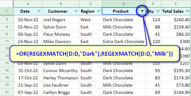
This is not the most advanced way though. There's also Google Sheets FILTER function that allows creating more complex conditions.
So, this is the standard Google Sheets filter with its options and custom formulas.
But let's change the task for a moment.
What if every employee required seeing only his/her sales? They would need to apply several filters in the same Google Sheets.
Is there a way to do that onle once, without recreating all over again?
Google Sheets Filter views will deal with the problem.
Google Sheets Filter views – create, name, save, and delete
Google Sheets Filter views help save filters for later in order to avoid recreating them again. They can be used by different users without interfering with each other.
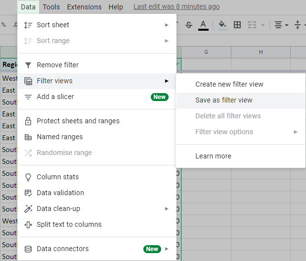
Since I already created a standard Google Sheets filter that I want to save for later, I click Data > Filter views > Save as filter view.
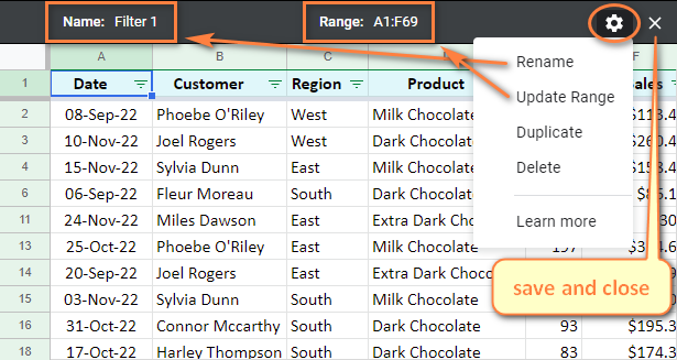
An additional black bar appears with the Options icon on its right. There you'll find the options to rename your filter in Google Sheets, update the range, duplicate it, or delete it completely. To save & close any Google Sheets filter view, click the Close icon at the upper right corner of the bar.
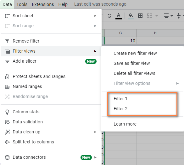
You can access and apply saved filters in Google Sheets anytime. I have only two of them:
One of the main advantages of Google Sheets is the possibility for several people to work with tables simultaneously. Now, imagine what may happen if different people wish to see different pieces of data.
As soon as one user applies a filter in his/her Google Sheets, other users will see the changes immediately, meaning the data they work with will become partially hidden.
To solve the problem, Filter Views option was created. It works on each user's side, so they could apply Google Sheets filters just for themselves without interfering with other's work.
To create a Google Sheets filter view, click Data > Filter views > Create new filter view. Then set the conditions for your data and name the view by clicking the "Name" field (or use the Options icon to rename it).
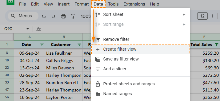
All the changes are saved automatically upon closing Filter Views. If they are no longer needed, remove them by clicking Options > Delete on the black bar.
Tip. If the spreadsheet owner permitted you to edit the file, all other users will be able to see and use filters created by you in Google Sheets.
Note. If all you can do is view the Google spreadsheet, you'll be able to create and apply Filter Views for yourself, but nothing will be saved upon closing the file. For that, you need permissions to edit the spreadsheet.
Easy way to filter by multiple conditions in Google Sheets (without formulas)
Filter in Google Sheets is one of the easiest features. Sadly, the number of conditions you can apply to one column at a time is scarcely enough to cover most of the tasks.
Custom formulas could provide a way out, but even they can be tricky to build correctly, especially for dates and time or with OR/AND logic.
Luckily, there’s a better solution – a special add-on for Google Sheets called Filter and Extract Data. It filters multiple rows and columns, each with lots of criteria applied. The extension is user-friendly, so you won’t have to doubt your own actions. But even if you do, the tool won’t alter your source data at all – it will copy and paste the filtered range wherever you decide. As a pleasant bonus, the add-on will deliver you from learning that scary Google Sheets VLOOKUP function ;)
Tip. Feel free to jump to the bottom of the page to see a video about the tool right away.
Once you install the add-on, you will find it under the Extensions tab in Google Sheets. The first step you’ll see is the only one there is:
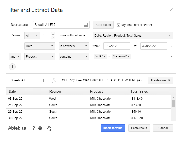
- Let’s use the add-on to filter my Google Sheets table of sales (A1:F69):

- The columns I’m really interested in are Date, Region, Product, and Total Sales, so I choose only them as the ones to return:

- Now it’s time to compose the conditions. Let’s try and get all sales of milk and hazelnut chocolate for September 2022:

- While you thread your criteria, the formula from the preview area at the bottom of the tool will modify itself accordingly. Click Preview result to peep at the found matches:
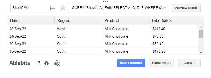
- Select the upper leftmost cells for the future filtered range and hit either Paste result (to return found matches as values) or Insert formula (to insert a formula with its outcome):
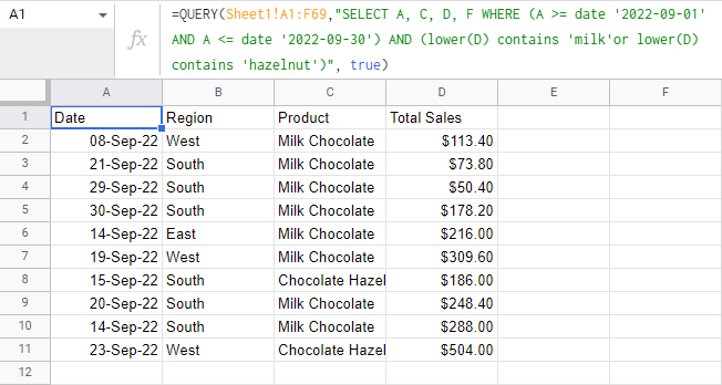
If you'd like to get to know Filter and Extract Data better, I encourage you to install it from the Google Workspace Marketplace or learn more about it on its home page.
Video: filter by multiple conditions, easy way
Filter and Extract Data is the best and the easiest way there is to filter your data in Google Sheets. Watch this demo video to learn all the benefits of owning the tool:
If you have any questions or you'd like to share some thoughts on filters in Google Sheets, feel free to leave a comment down below.
 by
by
31 comments
Hello I'd like to ask if we can filter view from conditional formatting.
I have a calendar which automatically recolors itself based on color using conditional formatting.
right now I have 3 color indicators
1. red for holidays and weekends.
2. orange for ongoing projects phase A.
3. blue for ongoing projects phase B.
is it possible for me to filter rows only to appear based on the color orange (due to conditional formatting)? the cell is of course, blank.
Hello Andrew C,
For me to be able to help you better, please share a small sample spreadsheet with us (support@apps4gs.com) with 2 sheets: (1) a copy of your source data (2) the result you expect to get. I kindly ask you to shorten the tables to 10-20 rows. I'll look into it and see if I can help.
Note. We keep that Google account for file sharing only and don't monitor its Inbox. Do not email there. Once you share the file, just confirm by replying to this comment.
Got it. I hope this can help. I've opened editor access to support@apps4gs.com
Thank you for sharing the file, Andrew.
You can't do that with the custom formula in the standard column filter because you'd have to get the formula for each column and it wouldn't work still. The conditions applied to several columns work simultaneously.
However, there's a way to return the required dataset to another place of your file with a formula. Please look at cell E26, I placed the formula there:
={E3:NF3; FILTER(CELLCOLOR(E4:NF19,"fill",TRUE), (INDEX(CELLCOLOR(E4:NF19,"fill",TRUE), 0, MATCH(TODAY(), E3:NF3, 0)) = "light yellow 2") + (INDEX(CELLCOLOR(E4:NF19,"fill",TRUE), 0, MATCH(TODAY(), E3:NF3, 0)) = "#b7e1cd"))}
It filters your original data by colored rows in the column with the today's date. Please note that formulas do not return colors. I put the colors you can see using conditional formatting rules, so check those as well to understand how it all works.
Hope this helps!
Thanks. Maybe I missed it but is there a simple way to dynamically display a filter of rows based on the active user email so with 1 FILTER VIEW it shows different ROWS based on the active user logged into the google sheet. (and of course each row within the google sheet that is active has a column that exactly matches the current logged in user email. )
Hello Fred,
Do you mean you'd like to see the filter view of the user who's using it now? With their email address somewhere in the table as well?
Hello,
Thanks for the post !
Useful!
Do you know how, with a filter on custom fomula limking ot the content of a cell, i have a dynamic view when the said content change ?
=$i3=$E$1
If I change the content of E1, I have to open again the filter and click on DONE again for it to actualize.
I get I can go with the function FILTER, but this is not convenient when you wants to actually modified the content inside the table.
Thank you for your feedback, Lycoeur!
For me to understand your task better, please share an editable copy of your sheet with me: support@apps4gs.com. If you have confidential information there, you can replace it with some irrelevant data, just keep the format. Please make sure your current filter is applied and specify what should be changed and where.
Note. We keep that Google account for file sharing only and don't monitor its Inbox. Please do not email there. Once you share the file, just confirm by replying to this comment.
I'll look into it and try to help.
I want to hide the rows with blank data and 1 column containing any value =0. I have tried with the filter view by conditions as well as value, but it is not static. I want to create that view for all the users of this google sheet. Please help.
Hello Biswadeep,
Filter View is only visible by the user who's applying it. It's your way to filter the data without changing it directly.
To filter the data so everyone could see it, use the standard Filter, not Filter view.
Hello,
you write here in article- when put condition into the CELL (instead of selecting condition in filtres directly): " Click the Filter icon on your Google Sheets column and then OK to update the results manually."
Is there a way how to do it AUTOMATICALY ? the update(refresh) step? because then it would be REALLY AWESOME
here is my simple sample data ....but i think that the question is clear at all.
thank you
https://docs.google.com/spreadsheets/d/1EQ83uSv0n5o3HtHcPTeIvpPCzfIYIMniL3XvhWtHwgs/edit#gid=145226926
Hello Dech,
We're always ready to help you, but we do not cover the programming area (script-related questions).
You may try to find a solution here – an overview of Google Apps Script with a lot of helpful content and links:
https://developers.google.com/apps-script/overview
I hope you’ll find this information helpful. Sorry I can't assist you better.
Hi Nat!
so i tried the script thing ....aaand - it is for me like seeeing the matrix code :-) so I tried how deep the rabit hole goes and it goes far... :)
shortly: after some week of research - I did it!!
there is no script that aupdates or refreshes the filter (to my knowledge) but there is a way how to SET UP the filter by script - so the script sets up the filter again and again - and actually you can call it "refresh" or "update" of filter
I have set TRIGGER to run the script everytime ANYTHING in the sheet changes (because i could find a way to trigger change in just one cell) and put my CONDITION of filter into some CELL (O1) - where i can change text according which is the data filtered
here is the code: https://developers.google.com/apps-script/reference/spreadsheet/filter-criteria-builder
function automaktfiltr() {
// Gets the existing filter on the sheet.
const ss = SpreadsheetApp.getActiveSheet();
let filter = ss.getFilter();
condition = ss.getRange("O1").getValue()
// Creates criteria that shows cells that contain "Northwest" and sets it to column B.
let criteria = SpreadsheetApp.newFilterCriteria()
.whenTextContains(condition)
.build();
filter.setColumnFilterCriteria(2, criteria);
}
Hi Dech,
Big thanks for sharing your solution on our blog! I believe it'll come in handy for other users with similar tasks :)
I have to face some problems with my Google sheets Data. I want to filter my google sheets data between two dates and also filter more conditions at the same time in the same sheets. Below are given some sample data.
https://docs.google.com/spreadsheets/d/1h5PW52PoMUxXtrqEmfXSCWu_OKXVO8IwUbHqcqSPRzs/edit?usp=share_link
Basically, I want to filter data between two dates & two more conditions at the same time in the same sheets.
Please help me with this issue.
Thanks
I am trying too hard to solve this issue but I can't solve this by myself. so if anyone solves this issue then please do this.
I'm very glad for all of you.
Thanks
Hello Shuvo,
I can see that you already have a working formula on the Solution sheet. The only thing I'd like to point out is that the formula is looking for the value from A13 in column D (Product details) while it should be column E (Category).
Thanks so much!
I'm having problems sharing a sheet that I want users to be able to filter/sort, but not edit (not change cell values). In your example above, you talk about having an employee filter to look at only *their* data in the sheet - this looks like my use case, where the manager enters the data and the employee can filter and see it, but not edit it. I seem to be missing some important step in how this all works because when I share the link with others, they can't access any filter views. Can you fill me in on what I'm missing here?
Hello JC,
When you share files and give users permissions to only view or comment on data, they can create their own filter views via Data > Filter views > Create new temporary filter vew. This menu is always accessible in spreadsheets. However, the users won't be able to see other users' filter views. Each user can create, save and see only his/her filter views.
Also, I'd recommend sharing the spreadsheet directly with users by adding their email addresses in the sharing settings.
Hello! Is it possible to filter by range, I try so
custom formula =ISNA(MATCH(B:B; Settings!D2:D200; 0))=FALSE
but for some reason it doesn't work.
Hello Max,
Please consider sharing your spreadsheet with us as well - support@4-bits.com. Once shared, please confirm by replying here since we don't monitor the Inbox of that email.
We'll look into it and try to help.
In $D$ i have some filed witch text.
Data table with filters I have from D31:D.
I add filter in custom formula =REGEXMATCH(D31:D;$D$3)
And it works.
But when I change data in D3 the results in my Table will refresh.
Eny idea how to refresh this data table?
Hi Tom,
Would you mind sharing a sample spreadsheet with us (support@4-bits.com) with your source data and the result you expect to get? We'd look into it.
Note. We keep support@4-bits.com for file sharing only and don't monitor its Inbox. Please do not email there. Once you share the file, just confirm by replying here.
Filter by, "Text Contains", is there an escape for the wildcards '*' and '?' ? Please include, or say there isn't, and offer the regex =REGEXMATCH(D:D,"\?")
Thanks!
Thank you very much for your feedback, John. :)
The formula wasn't mentioned intentionally since:
1) it works with textual values only, meaning the users would have to wrap their numbers in the TEXT function and then with the one you suggested.
2) wildcard characters cannot be used in your formula. It looks for the exact sequences you indicate in "". Thus "\?" won't find anything since we don't have this in our cells.
3) the function is case-sensitive and won't find anything if I enter "d" for all these "Dark Chocolate" cells.
4) all of the above make the formula too complicated to use, leaving the easiest option of wildcard characters.
Great explanation! I especially appreciate that you have shown equivalent custom formulas for the built-in criteria like 'Text contains', useful as a starting point for more complex criteria.
One possible correction: you state "Note. The formula can refer only to the column it's applied to..." but it appears that has changed. Today I was able to apply this formula with success: =OR(A:A="horses",C:C="cat") referring to two different columns. This worked regardless of whether I attached this custom formula to column A or column C.
This is a significant improvement for me, because it appears (to be tested...) that it will enable quite complex multi-column criteria, combined with the advantage that the filtered data can be edited, apparently not the case with results from QUERY( or FILTER(.
Thank you for your feedback, Chris.
Unfortunately, the formula like you provided doesn't work for me. However, if I take the formula where I refer to column B in both conditions and apply it to column E - it works. Thank you for pointing that out.
Thank you. Your article helped me. Have a nice day and Happy New 2019 Year! :)
the below link is shared publicly
https://docs.google.com/spreadsheets/d/1hWGAaDTnR_08OcB950dPczHpjvuHyVpohghOQD8QTW4/edit?usp=sharing
If someone could help me come up with a filter that shows any occurrence of the word Blue in either Column B OR Column C
Thank You in advance.
pehn di lann, assi khotte haan, assi kanjar haan.
I want to create a spreadsheet that references a column for a specific suffix, then have it take data from another cell in a row that contains said suffix and total it in another cell.ia that possible?