When you analyze your tables in Google Sheets, very often you need only a part of the information, while the table may contain dozens of various datasets. What's more, a bunch of various values may simply interfere.
Sure, you can always duplicate the table and delete those temporarily unwanted values. But isn't it a waste of time?
That is when Google Sheets filters lend a helping hand.
So, what is a "filter"? It's one of many Google Sheets options that lets you hide a part of data that you don't need at the moment. This way you don't need to delete the data. You simply hide it temporarily and can display it back any time.
Besides, this enables you to sort the data. Isn't that a pleasant perk? ?
How to filter your data in Google Sheets?
To filter your table, you need to select the range of interest manually. But something tells me you have loads of data.
So, to do the job faster, I advise you to select entire columns. I explained how to do that in one of my previous articles.
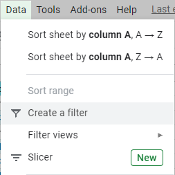
If you want to filter the entire table, just click its any cell and go to Data > Create a filter right away:
Or simply use a corresponding button on the Google Sheets toolbar:
![]()
Note. When you enable Google Sheets filter, it will work only for columns with data. If you have completely empty columns, the filter won't treat them as part of your table. You can include them by selecting the range with these columns manually.
Tip. You may want to lock the first row of the table that contains filter buttons. This way you won't have to scroll all the way up to adjust filter settings.
So, the filter is there. Each column header contains kind of an upside-down pyramid icon meaning that the table can now be filtered.
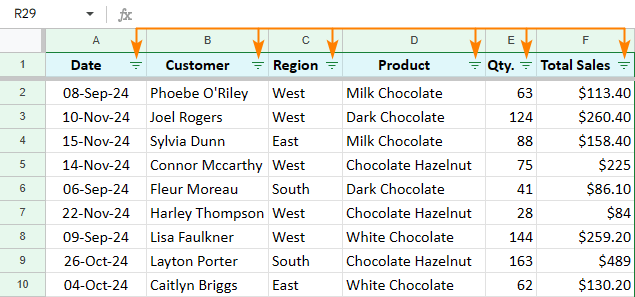
Now, let's try and adjust it.
Filter by values in Google Sheets
Let's start with the most basic filter option – filter by value. Decide by which column you'd like to filter first and click that pyramid icon next to the column header:
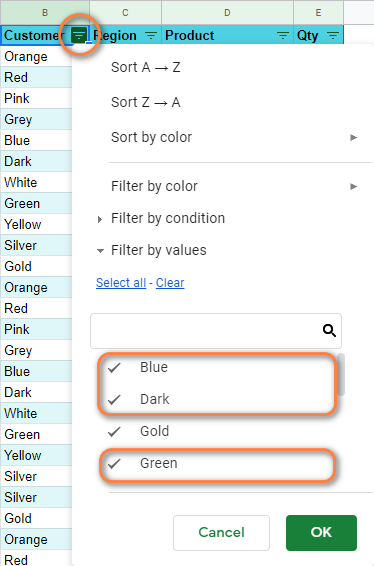
Uncheck all the values you want to hide temporarily and click OK.
You'll notice that some of the data has disappeared from the screen right away. Don't worry, the entries weren't deleted. They are there, in your table, you just don't see them because of the Google Sheets filter.
You can sort the remained values either A to Z or Z to A:
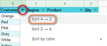
Tip. The filter icon changes next to those column headers where the filter is applied.
If necessary, you can always set additional filters. I'll do it with the Product column, to see the information about Dark and Extra Dark Chocolate only:
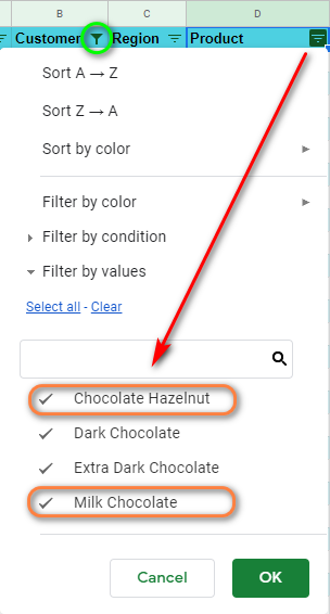
As a result, both filters are applied to the whole table and there are even fewer entries than before:
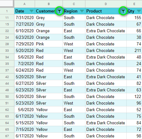
The rows we see now meet our two requirements.
Filter by color in Google Sheets
It may very well be that you use different font and background colors to present your data in the best and self-explanatory way possible. For cases like this, there’s another extremely useful option available in Google Sheets – filter by color.
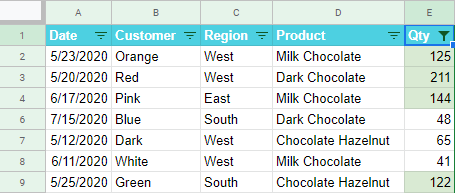
For example, here I have a list of purchased items per order. My conditional formatting rules dictate the following: if the number of items is less than 40, the number is colored red. If greater than or equal to 100, the fill color is green:
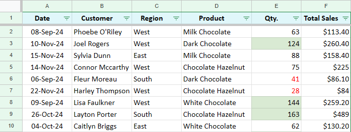
Let's apply Google Sheets filters to this table.
Option 1. Filter by text color in Google Sheets
I'm going to filter data by font color and hide all records but those in black:
- Apply the filter to your table first.
- Then click the pyramid icon in the column to filter by and select Filter by color > Text Color > black:
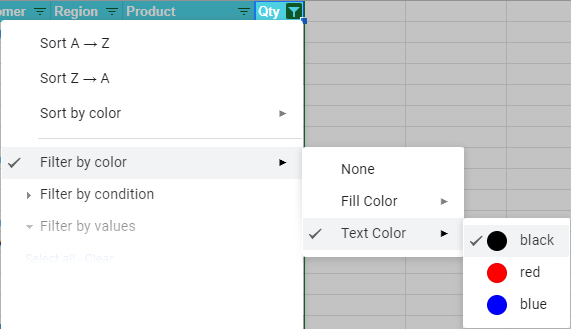
Note. Only the rows with the color you select will remain in the table. Other rows will be hidden. So make sure to choose the color that you want to see in your table.
As you can see, all records with any text color but black have been filtered:
Option 2. Filter by fill color in Google Sheets
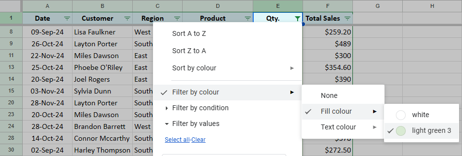
Another way would be to filter by fill color in Google Sheets. I can filter the table and keep only rows with the green background color with the following: Filter by color > Fill Color > light green 3:
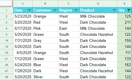
Now I see only rows where Qty cells are colored green:
Note. At the moment, Google Sheets allows neither filtering by both fill and text color nor filtering by several font hues/background hues.
Option 3. Remove all filters by color
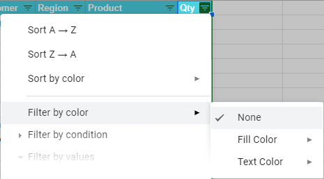
To remove any filtering by color simply go to Filter by color > None, and all formerly filtered rows will appear anew:
So, filtering the table by values or colors is not rocket science. But will it be enough for the list of 100+ entries and a bunch of parameters to consider?
In cases like this, I believe, you'd better apply filters by conditions in Google Sheets. There's even a super tool for the task – the knowledge of absolutely no formula is required. ;)
In addition, that article will teach you how to share different filtering results with different people within one document.
 by
by
10 comments
Hello;
Enjoy your tips... I have lost the menu selection CREATE FILTER" under the DATA menu item n ... in one Google Sheet ? what is happening ? I use all the time in both Excel and Sheets ...
I deleted all Filter Views, and cannot make the Create Filter work, since it is gone.
Thanks
Hello Marc,
Regarding your problem, please turn to Google support service for assistance:
open your spreadsheet and click Help > Report a problem. Then follow the instructions in the Send feedback window.
I wish I could help you better.
I am Very happy your information.
I am trying to filter out some data but only if the 2 columns passed a certain condition. Ex I wanted to eliminate all the zero in column A if column B is also zero. If its only column A that's zero or column B then I dont want it to be filtered out. Can you help me solve this problem? Please! I am trying the custom formula in the filters but i just dont know what formula to use. Please help!
Marilou,
The custom formula that helped me with this task is:
=OR(A:A<>0,B:B<>0)
Please refer to this article to filter by conditions correctly.
I am unable to get this simple task to work and was hoping you might be able to shed some light.
Google Help "Filter your data":
Search: Search for data points by typing in the search box. For example, typing "??" will shorten your list to just the cells that contain "??".
Hi Dan,
To see only values that contain "??", first, pick the "Clear" option to unselect all values from a filter search. Then enter ?? into the filter search field and make sure the value is checked.
Hope this makes at least a bit clear how to filter the values.
And the award for the worst UX in the world goes to...
Google Sheets column filters for their incredible work on the "Clear then search then Select All" behaviour.
Using the formula:
=ArrayFormula($D$2&""&TEXT(ROW(A1:A10000),"00000"))
- Where $D$2 is the constant number 4017 1501 100
- Row (A1:A10000) creates 10,000 numbers in sequence (1 - 10,000)
- The text function (that wraps the row function) creates leading zeros's thus 1 is displayed as 00001
- The Array function (Entering Ctrl+Shift+Enter) allows you to create 1 formula and apply it for the entire range (10,000 values in this case)
Look through the shared Google Sheets link for more info: https://docs.google.com/spreadsheets/d/19Wx1plSbARg8ZoFeeEn11Zls9nA3odRMFi9aHVylRns/edit?usp=sharing
Hello,
I have to send my printer a bunch of promo codes, 10,000 to be exact. I'm trying to send him a file from Google Sheets. So the first number would be 4017 1501 100 00001, the 2nd number would all be the same except the last or 00002, and so on to 4017 1501 100 10000. Can this be done?
Thanks so much,
Kevin