The tutorial shows how to use the PERCENTOF function in Excel. It includes practical examples of percentage of total formulas to help you understand how they work in real data.
Calculating how much each value contributes to a total is something many Excel users do every day. In older versions, this usually meant creating your own formula that divided a part by the whole. The PERCENTOF function gives you a quick and direct way to return that percentage without building a formula manually. In this article, you'll learn the inner mechanics of the function and how to use it effectively in your own worksheets.
Excel PERCENTOF function
The PERCENTOF function in Excel is used to calculate what percentage a given subset contributes to the whole. Put simply, it shows how much of the entire dataset a specific value or group of values accounts for.
You provide two inputs, the part (subset) and the whole (all data), and the function returns the result as a decimal value that can be formatted as a percentage.
The syntax of the PERCENTOF function is as follows:
Where:
- data_subset – the portion of data that makes up part of the total. This can be a single number, a cell reference, a range, or an array.
- data_all – the complete dataset, provided as a range or array.
Both arguments are required.
How it works
The PERCENTOF function operates by comparing the sum of a subset to the sum of all values. Mathematically, it's equivalent to using this formula:
=SUM(data_subset) / SUM(data_all)
Excel performs this calculation behind the scenes, saving you time and reducing the chance of formula errors in your worksheets.
Availability
The PERCENTOF function is only available in Excel for Microsoft 365. It is not supported in earlier Excel versions, where equivalent calculations can be performed with a classic percentage formula.
Basic PERCENTOF formula for percentage of total in Excel
To get familiar with how the PERCENTOF function works, let's start with a simple example. Imagine you have a list of monthly expenses in C3:C21, and you want to find out what portion each cost takes from the full budget. For this, we use the following formula:
=PERCENTOF(C3, $C$3:$C$21)
Here, C3 is a subset of data (a single cost) and $C$3:$C$21 is the full set of expenses (the total).
Copy the formula down the column, and you will get a list of decimal numbers, as shown in the screenshot below:
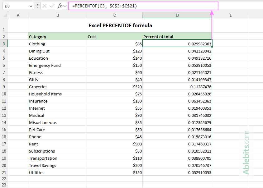
To convert these decimals into percentages:
- Select all the result cells (D3:D21).
- Click the % icon on the Home tab in the Number group.
- Use the Increase Decimal or Decrease Decimal buttons to adjust the number of decimal places as desired.
Now that you have the results properly formatted, you can sort by the Percent column to quickly see which expenses take up the largest share of your budget.
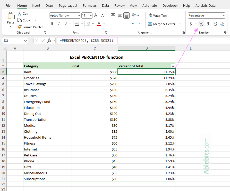
The same result can be achieved by calculating the total separately (say, in cell C23) and referencing that cell in the second argument of PERCENTOF:
=PERCENTOF(C3, $C$23)
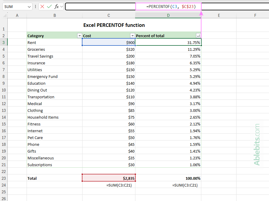
To confirm your calculations, sum up all percentages with this formula in D23:
=SUM(D3:D21)
If everything is correct, the total should equal 100% 😊
Excel PERCENTOF function - usage notes
To ensure your PERCENTOF calculations always stay accurate, keep these points in mind:
- When copying the formula down multiple rows, lock the reference to your total, either a single cell (like $C$23) or a range (such as $C$3:$C$21), so it doesn't shift.
- Make sure your total represents the full dataset; missing a value will skew every percentage.
- If the full range is empty or could potentially be zero, consider wrapping the formula in the IF function to prevent divide-by-zero errors:
=IF(SUM($C$3:$C$21)=0, "", PERCENTOF(C3, $C$3:$C$21))
How to use PERCENTOF in Excel – formula examples
While PERCENTOF is useful on its own, it becomes even more helpful when combined with Excel's dynamic array aggregation functions. In fact, it was designed to complement these functions, allowing you to display individual data parts as percentages of the total within summarized results.
Using PERCENTOF with GROUPBY function
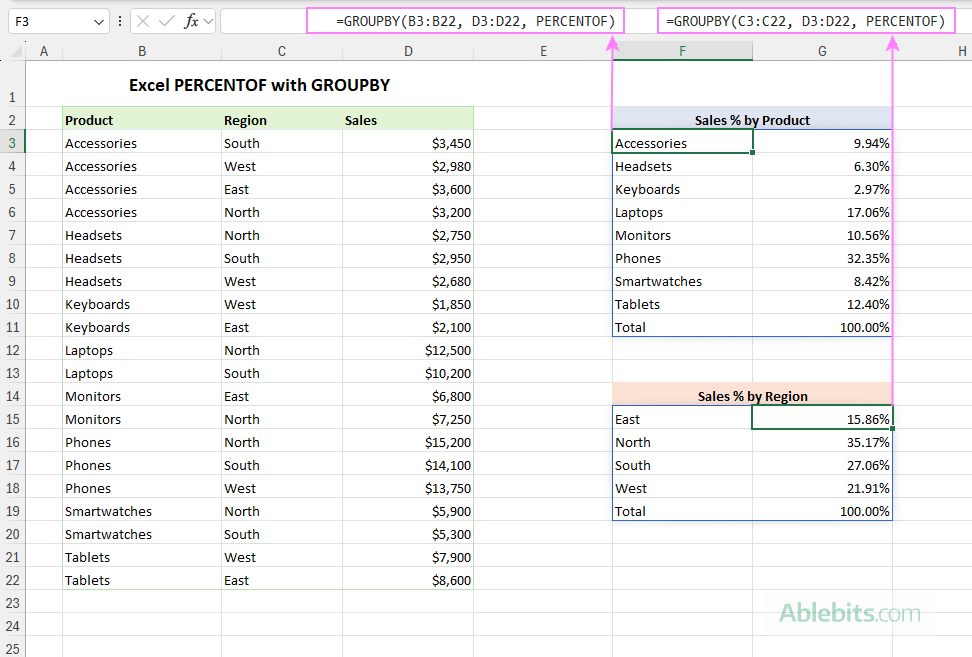
A GROUPBY formula with nested PERCENTOF lets you break data into categories and return each group's share of the total as percentages. Here's how it works in practice:
Suppose you have products in column B, regions in column C, and sales numbers in column D.
To find out what portion of total sales each product represents, use this formula:
=GROUPBY(B3:B22, D3:D22, PERCENTOF)
To get each region's share, use this one:
=GROUPBY(C3:C22, D3:D22, PERCENTOF)
Remember to format the returned decimal numbers as percentages, and you will clearly see how much each product or region contributes to the overall sales:
Using PERCENTOF with PIVOTBY function
When your analysis calls for grouping data by both rows and columns, PIVOTBY is the formula to use. With PERCENTOF as the summary function, it returns each row-column combination as a percentage of the total, presented in a familiar pivot table layout.
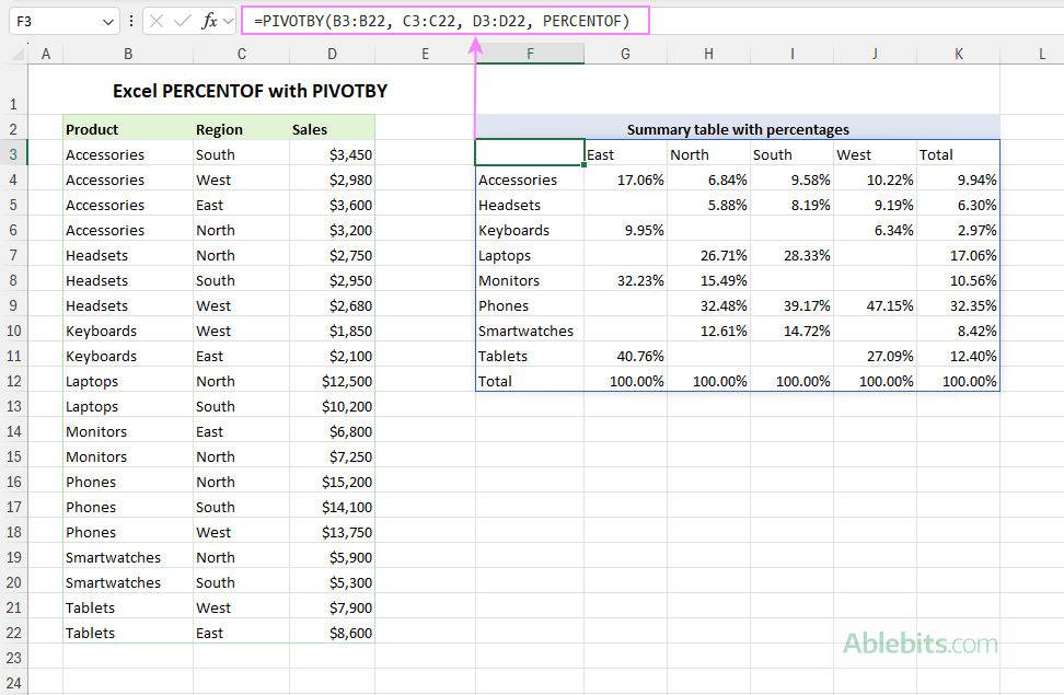
In the example below, products are grouped in rows, regions in columns, and the sales amounts are summarized. To create this kind of summary table, the formula is:
=PIVOTBY(B3:B22, C3:C22, D3:D22, PERCENTOF)
Calculating percentage of non-numeric values
In all the previous examples, we worked with numbers. But what if your worksheet only contains text values and you still want to know the percentage each item represents in the dataset?
For example, imagine you have a list of event attendees and their countries, and you'd like to find what share each country represents.
A GROUPBY formula with COUNTA handles the counts easily:
=GROUPBY(C3:C22, C3:C22, COUNTA)
Here, C3:C22 are country names, and the formula returns how many times each country appears in the list.
But a similar attempt to calculate percentages fails:
=GROUPBY(C3:C22, C3:C22, PERCENTOF)
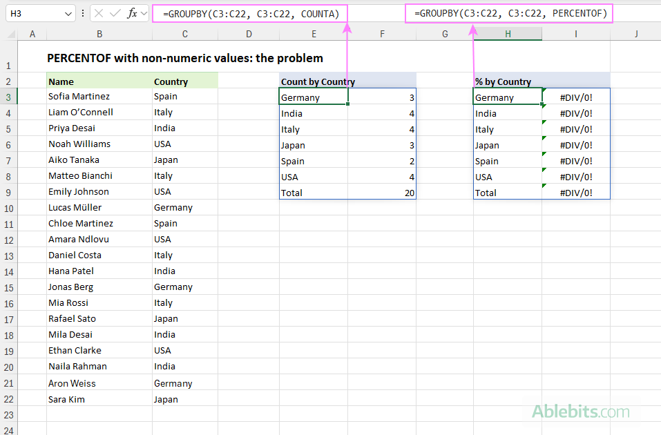
This happens because the logic behind PERCENTOF implies calculating numbers:
=SUM(subset) / SUM(all_data)
When Excel tries to sum text values like country names, it can't compute totals and returns a #DIV/0! error.
For PERCENTOF to work, the second argument of GROUPBY, named values, must be a numeric array. And there are several easy ways to create one in Excel.
Formula 1: Use an existing numeric column
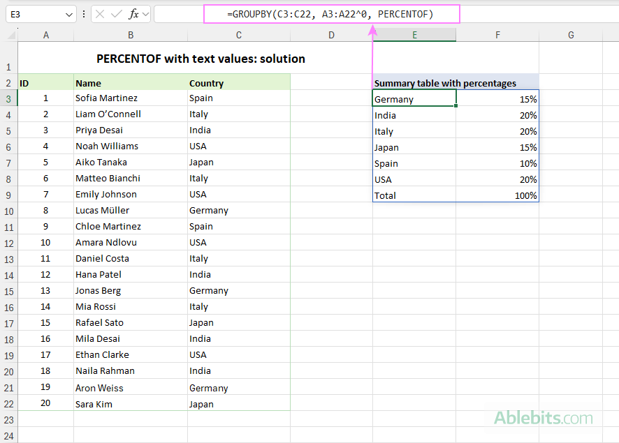
If your dataset already contains any numeric column (for example, ID numbers in A3:A22), you can turn that column into an array of 1s by raising each value to the power of zero:
=GROUPBY(C3:C22, A3:A22^0, PERCENTOF)
Since any number raised to the power of zero equals 1, an array like {1;1;1;…1} gets to the values argument. GROUPBY then counts how many 1s belong to each country and returns the percentage for each group.
Formula 2: Generate a numeric sequence
If your dataset has no numeric column at all, you can use the SEQUENCE function to generate an array of 1s matching the length of your dataset:
=SEQUENCE(ROWS(C3:C22),,1,0)
The complete formula becomes:
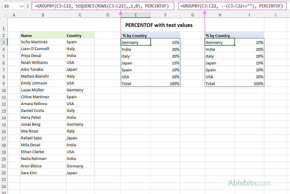
=GROUPBY(C3:C22, SEQUENCE(ROWS(C3:C22),,1,0), PERCENTOF)
As with the previous method, this assigns a numeric value of 1 to each country, allowing PERCENTOF to compute group percentages.
Formula 3: Convert text values to numbers
Another way to create a required array is by using a logical expression: --(C3:C22<>"")
This checks whether each cell in the specified range is not empty. TRUE and FALSE are then converted to 1 and 0 using the double unary operator (--).
In our case, every non-blank country name becomes a 1, so we get a numeric array exactly as needed. Using it in GROUPBY produces the same result as the previous formulas:
=GROUPBY(C3:C22, --(C3:C22<>""), PERCENTOF)
Now that you know how the PERCENTOF function works with numbers, text values, and dynamic arrays, you can start applying it to your own worksheets to reveal trends that raw values can't always show. For hands-on practice, feel free to download our sample workbook and experiment with how the function behaves in grouped and pivoted results.
Practice workbook for download
Excel PERCENTOF formula examples (.xlsx file)
 by
by