In this article, you will learn various ways to concatenate text strings, numbers and dates in Excel using the CONCATENATE function and "&" operator. We will also discuss formulas to combine individual cells, columns and ranges.
In your Excel workbooks, the data is not always structured according to your needs. Often you may want to split the content of one cell into individual cells or do the opposite - combine data from two or more columns into a single column. Common examples are joining names and address parts, combining text with a formula-driven value, displaying dates and times in the desired format, to name a few.
In this tutorial, we are going to explore various techniques of Excel string concatenation, so you can choose the method best suited for your worksheets.
What is "concatenate" in Excel?
In essence, there are two ways to combine data in Excel spreadsheets:
- Merging cells
- Concatenating cells' values
When you merge cells, you "physically" join two or more cells into a single cell. As a result, you have one larger cell that is displayed across multiple rows and/or columns.
When you concatenate cells in Excel, you combine only the contents of those cells. In other words, concatenation in Excel is the process of joining two or more values together. This method is often used to combine a few pieces of text that reside in different cells (technically, these are called text strings or simply strings) or insert a formula-calculated value in the middle of some text.
The following screenshot demonstrates the difference between these two methods:

Merging cells in Excel is the subject of a separate article, and in this tutorial, we'll discuss the two main ways to concatenate strings in Excel - by using the CONCATENATE function and the concatenation operator (&).
Excel CONCATENATE function
The CONCATENATE function in Excel is used to join different pieces of text together or combine values from several cells into one cell.
The syntax of Excel CONCATENATE is as follows:
Where text is a text string, cell reference or formula-driven value.
The CONCATENATE function is supported in all versions of Excel 365 - 2007.
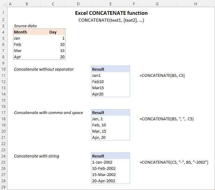
For example, to concatenate the values of B6 and C6 with a comma, the formula is:
=CONCATENATE(B6, ",", C6)
More examples are shown in the image below:
Note. In Excel 365 - Excel 2019, the CONCAT function is also available, which is a modern successor of CONCATENATE with exactly the same syntax. Although the CONCATENATE function is kept for backward compatibility, Microsoft does not give any promises that it will be supported in future versions of Excel.
Using CONCATENATE in Excel - things to remember
To ensure that your CONCATENATE formulas always deliver the correct results, remember the following simple rules:
- Excel CONCATENATE function requires at least one "text" argument to work.
- In one formula, you can concatenate up to 255 strings, a total of 8,192 characters.
- The result of the CONCATENATE function is always a text string, even when all of the source values are numbers.
- Unlike the CONCAT function, Excel CONCATENATE does not recognize arrays. Each cell reference must be listed separately. For example, you should use CONCATENATE(A1, A2, A3) and not CONCATENATE(A1:A3).
- If any of the arguments is invalid, the CONCATENATE function returns a #VALUE! error.
"&" operator to concatenate strings in Excel
In Microsoft Excel, the ampersand sign (&) is another way to concatenate cells. This method comes in very handy in many scenarios since typing an ampersand is much faster than typing the word "concatenate" :)
For example, to concatenate two cell values with a space in-between, the formula is:
=A2&" "&B2
How to concatenate in Excel - formula examples
Below you will find a few examples of using the CONCATENATE function in Excel.
Concatenate two or more cells without separator
To combine the values of two cells into one, you use the concatenation formula in its simplest form:
=CONCATENATE(A2, B2)
Or
=A2&B2
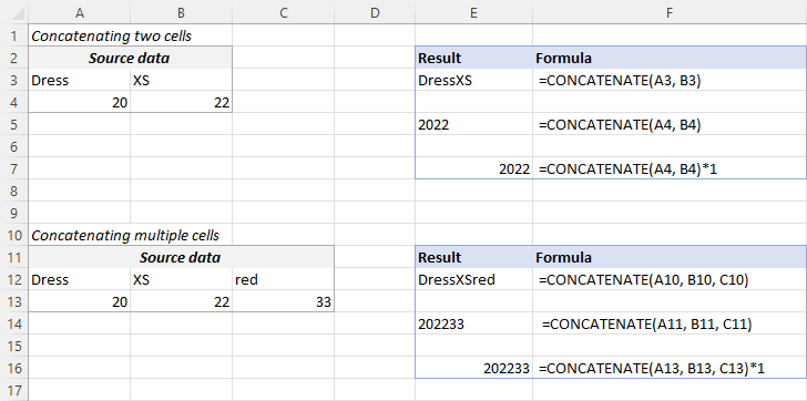
Please note that the values will be knit together without any delimiter like in the screenshot below.
To concatenate multiple cells, you need to supply each cell reference individually, even if you are combining contiguous cells. For example:
=CONCATENATE(A2, B2, C2)
Or
=A2&B2&C2
The formulas work for both text and numbers. In case of numbers, please keep in mind that the result is a text string. To convert it to number, just multiply CONCATENATE's output by 1 or add 0 to it. For instance:
=CONCATENATE(A2, B2)*1
Tip. In Excel 2019 and higher, you can use the CONCAT function to quickly concatenate multiple cells using one or more range references.
Concatenate cells with a space, comma or other delimiter
In your worksheets, you may often need to join values in a way that includes commas, spaces, various punctuation marks or other characters such as a hyphen or slash. To do this, simply put the desired character in your concatenation formula. Remember to enclose that character in quotation marks, as demonstrated in the following examples.
Concatenating two cells with a space:
=CONCATENATE(A2, " ", B2)
or
=A2 & " " & B2
Concatenating two cells with a comma:
=CONCATENATE(A2, ", ", B2)
or
=A2 & ", " & B2
Concatenating two cells with a hyphen:
=CONCATENATE(A2, "-", B2)
or
=A2 & "-" & B2
The following screenshot demonstrates how the results may look like:

Tip. In Excel 2019 and higher, you can use the TEXTJOIN function to merge strings from multiple cells with any delimiter that you specify.
Concatenating text string and cell value
There is no reason for the Excel CONCATENATE function to be limited to only joining cells' values. You can also use it to combine text strings to make the result more meaningful. For example:
=CONCATENATE(A2, " ", B2, " completed")
The above formula informs the user that a certain project is completed, as in row 2 in the screenshot below. Please notice that we add a space before the word " completed" to separate the concatenated text strings. A space (" ") is also inserted between the combined values, so that the result displays as "Project 1" rather than "Project1".
With the concatenation operator, the formula can be written this way:
=A2 & " " & B2 & " completed"
In the same manner, you can add a text string in the beginning or in the middle of your concatenation formula. For example:
=CONCATENATE("See ", A2, " ", B2)
="See " & A2 & " " & B2

Join text string and another formula
To make the result returned by some formula more understandable for your users, you can concatenate it with a text string that explains what the value actually is.
For example, you can use the following formula to return the current date in the desired format and specify what kind of date that is:
=CONCATENATE("Today is ",TEXT(TODAY(), "mmmm d, yyyy"))
="Today is " & TEXT(TODAY(), "dd-mmm-yy")

Tip. If you would like to delete the source data without affecting the resulting text strings, use the "Paste special - values only" option to convert formulas to their values.
Concatenate text strings with line breaks
Most often, you would separate the resulting text strings with punctuation marks and spaces, as shown in the previous example. In some cases, however, there may be a need to separate the values with a line break, or carriage return. A common example is merging mailing addresses from data in separate columns.
A problem is that you cannot simply type a line break in the formula like a usual character. Instead, you use the CHAR function to supply the corresponding ASCII code to the concatenation formula:
- On Windows, use CHAR(10) where 10 is the character code for Line feed.
- On Mac, use CHAR(13) where 13 is the character code for Carriage return.
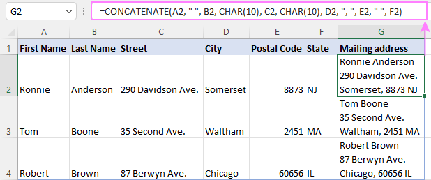
In this example, we have the address pieces in columns A through F, and we are putting them together in column G by using the concatenation operator "&". The merged values are separated with a comma (", "), space (" ") and a line break CHAR(10):
=A2 & " " & B2 & CHAR(10) & C2 & CHAR(10) & D2 & ", " & E2 & " " & F2
The CONCATENATE function would take this shape:
=CONCATENATE(A2, " ", B2, CHAR(10), C2, CHAR(10), D2, ", ", E2, " ", F2)
Either way, the result is a 3-line text string:
In the same manner, you can separate final strings with other characters such as:
- Double quotes (") - CHAR(34)
- Forward slash (/) - CHAR(47)
- Asterisk (*) - CHAR (42)
- The full list of ASCII codes is available here.
How to concatenate columns in Excel
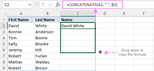
To join two or more columns, just enter your concatenation formula in the first cell, and then copy it down to other cells by dragging the fill handle (the small square that appears in the lower right hand corner of the selected cell).
For example, to combine two columns (column A and B) delimiting the values with a space, the formula in C2 copied down is:
=CONCATENATE(A2, " ", B2)
Or
= A2 & " " & B2
For more information, please see How to merge two columns in Excel without losing data.
Combine text and numbers keeping formatting
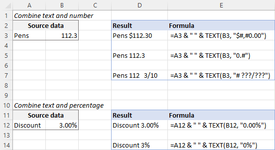
When concatenating a text string with a number, percentage or date, you may want to keep the original formatting of a numeric value or display it in a different way. This can be done by supplying the format code inside the TEXT function, which you embed in a concatenation formula.
In the beginning of this tutorial, we have already discussed a formula that concatenates text and date.
And here are a few more formula examples that combine text and number:
Number with 2 decimal places and the $ sign:
=A2 & " " & TEXT(B2, "$#,#0.00")
Number without insignificant zeros and the $ sign:
=A2 & " " & TEXT(B2, "0.#")
Fractional number:
=A2 & " " & TEXT(B2, "# ?/???")
To concatenate text and percentage, the formulas are:
Percent with two decimal places:
=A12 & " " & TEXT(B12, "0.00%")
Rounded whole percent:
=A12 & " " & TEXT(B12, "0%")
How to concatenate a range of cells in Excel
Combining values from multiple cells might take some effort because the Excel CONCATENATE function does not accept arrays.
To concatenate several cells, say A1 to A4, you need to use one of the following formulas:
=CONCATENATE(A1, A2, A3, A4)
or
=A1 & A2 & A3 & A4
When combining a fairly small group of cells, it's no big deal to type all the references. A large range would be tedious to supply, typing each individual reference manually. Below you will find 3 methods of quick range concatenation in Excel.
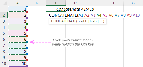
Method 1. Press CTRL to select multiple cells
To quickly select several cells, you can press and hold the Ctrl key while clicking on each cell you want to include in the formula. Here are the detailed steps:
- Select a cell where you want to enter the formula.
- Type =CONCATENATE( in that cell or in the formula bar.
- Press and hold Ctrl and click on each cell you want to concatenate.
- Release the Ctrl button, type the closing parenthesis, and press Enter.
Method 2. Use TRANSPOSE function to get all cell values
When a range consists of tens or hundreds of cells, the previous method may not be fast enough as it requires clicking on each cell. In this case, you can use the TRANSPOSE function to return an array of values, and then merge them together in one fell swoop.
- In the cell where you want the result to appear, enter the TRANSPOSE formula, for example:
=TRANSPOSE(A1:A10)
- In the formula bar, press F9 to replace the formula with calculated values. As a result, you will have an array of values to be concatenated.
- Delete the curly braces surrounding the array.

- Type =CONCATENATE( before the first value, then type the closing parenthesis after the last value, and press Enter.

Note. The result of this formula is static as it concatenates the values, not cell references. If the source data changes, you will have to repeat the process.
Method 3. Use the CONCAT function
In Excel 365 and Excel 2021, this simple formula will concatenate a range of cells in a blink:
=CONCAT(A1:A10)
Method 4. Use the Merge Cells add-in
A quick and formula-free way to concatenate any range in Excel is to use the Merge Cells add-in with the "Merge all areas in selection" option turned off, as demonstrated in Combining values of several cells into one cell.
Excel "&" operator vs. CONCATENATE function
Many users wonder which is a more efficient way to join strings in Excel - CONCATENATE function or "&" operator.
The only real difference is the 255 strings limit of the CONCATENATE function and no such limitation when using the ampersand. Other than that, there is no difference between these two methods, nor is there any speed difference between the CONCATENATE and "&" formulas.
And since 255 is a really big number and you will hardly ever need to combine that many strings in real work, the difference boils down to comfort and ease of use. Some users find CONCATENATE formulas easier to read, I personally prefer using the "&" method. So, simply stick with the technique you feel more comfortable with.
Opposite of CONCATENATE in Excel (splitting cells)
The opposite of concatenate in Excel is splitting the contents of one cell into multiple cells. This can be done in a few different ways:
- Text to Columns feature
- Flash Fill option in Excel 2013 and higher
- TEXTSPLIT function in Excel 365
- Custom formulas to split cells (MID, RIGHT, LEFT, etc.)
You can also find useful information in this article: How to unmerge cells in Excel.
Concatenate in Excel with Merge Cells add-in
With the Merge Cells add-in included in Ultimate Suite for Excel, you can efficiently do both:
- Merge several cells into one without losing data.
- Concatenate the values of several cells into a single cell and separate them with any delimiter of your choosing.
The Merge Cells tool works with all Excel versions from 2016 to 365 and can combine all data types including text strings, numbers, dates and special symbols. Its two key advantages are simplicity and speed - any concatenation is done in a couple of clicks.
Combine values of several cells into one cell
To combine the contents of several cells, you select the range to concatenate and configure the following settings:
- Under What to merge, select Cells into one.
- Under Combine with, type the delimiter (a comma and a space in our case).
- Choose where you want to place the result.
- Most importantly, uncheck the Merge all areas in the selection box. It is this option that controls whether the cells are merged or their values are concatenated.

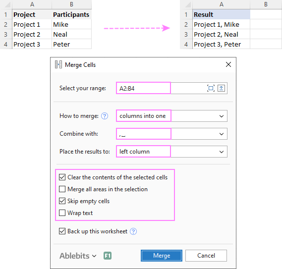
Combine columns row-by-row
To concatenate two or more columns, you configure the Merge Cells' settings in a similar way but choose to merge columns into one and place the results in the left column.
Join rows column-by-column
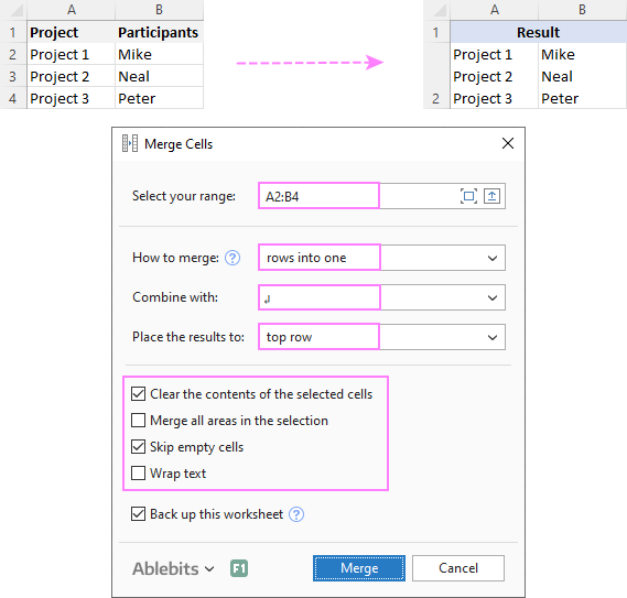
To combine data in each individual row, column-by-column, you choose:
- Merge rows into one.
- Use a line break for the delimiter.
- Place the results in the top row.
The result may look similar to this:
To check how the Merge Cells add-in will cope with your data sets, you are welcome to download a fully functional trial version of our Ultimate Suite for Excel below.
That's how to concatenate in Excel. I thank you for reading and hope to see you on our blog next week!
Available downloads
Concatenation formula examples (.xlsx file)
Ultimate Suite 14-day trial version (.exe file)
 by
by
447 comments
I may not know the right word to use pls pardon me:
My name is Apple
Joy
Peace
goodness
love
sound
mind
I want Column 1(My name is) to be linked with each of the Column 2 (name list) above in a new column(Column 3) Thanks
I want to use a concatenation formula. Pulling information for several cells the cells either have a date for example cell F4 or are left blank. I want the formula to pick up the date or put in “no date at this time” and I’m not sure how to make the formula work.
I want to use a concatenation formula. Pulling information for several cells the cells either have a date for cell F or are left blank. I want the formula to pick up the date or put in “no date at this time” and I’m not sure how to make the formula work.
Elizabeth:
Will this work?
Test to see if cell is empty, if it is then return "No Date At This Time", otherwise return the cell's contents.
Where the data is in cell A18, it looks like this:
=IF(ISBLANK(A18),"No Date at this time",A18)
Mr.Doug
Thank you for reply
but i want result is 010155
this result is 1155
That sounds like a cell formatting issue.
Select the cells and choose format cells and then choose custom and use one of the provided formats or use one as a starting point and then change it to the format you want.
I want to concat A1 cell value 01
B1 cell value 05
c1 cell value 5
how to concat
I want result d1 cell 01055
Please reply me
D1=Concatenate(A1,b1,c1)
COL1 COL2
1 AAA
1 GGG
1 FFF
2 GGG
2 HHH
3 RRR
3 JJJ
concatenate text based on criteria in Excel? FORMULAS
Not sure what the criteria is, but here's a way to do this.
If numbers are in cells A1 through A10 and letters are in cells B1 through B10 and your criteria is if a cell contains a "1" then:
=IF(OR(A1=1,A2=1,A3=1,(Concatenate(B1," ",B2," ",B3))
thanks for the support
Thank you!
While I'm pretty sue, that there is an easier way to do what I need (replace input value with text including said value), probably even in single column (yet no tutorial, how to do that, with concatenate function I achieved my goal:
=CONCATENATE("OAM-";C2;"/PP-2017")
And even expanded it for future use (albeit at the cost of 2 extra columns *sad*):
=CONCATENATE("OAM-";C2;"/";D2;"-201";E2)
Result (where XXXXX is the input number):
OAM-XXXXX/PP-2017
Hello!
How do I concatenate based a number such as...
N = 5
String = "Hello"
Desired output = "xxxxxHello"
N = 3
String = "Hello"
Desired output = "xxxHello"
Thanks
here is one i am trying to do...
I have a pricing matrix and i have named each cell in the matrix by its location within the matrix, example...
A1=ABa1, B1=ABa2, C1=ABa3
A2=ABb1, B2=ABb2, C2=ABb3
A3=ABc1, B3=ABc2, C3=ABc3
so on another sheet i have my products that are coded with these name. example...
Product A: S1234a1
Product B: S4567b4
i want to strip that "a1" off the end and then use it in the formula to show the price for ABa1.
I use "RIGHT" formula to grab the 'a1' text, and then i use CONCATENATE with plain AB text to create the value ABa1 displayed in the cell. so thats great i can see a string on data that is exactly what i want
so heres my dilemma...
in any cell, if i manually type in "=ABa1", it refers to the cell which i named ABa1 and the value within that cell is displayed. makes sense works perfect...
but what i want to do is use my CONCATENTATED string of data, rather that actually keying in the my "=ABa1".
somehow like this....=(the concatenated data string i want use), and then will have the same affect as when i manually key it in.
Thank you for this excellent guide. I have a series of concatenated sentences each with text intermixed with values (numbers) pulled from other cells. In some cases, I have used the TEXT function to render the desired number format. However, I am looking to make the values (whether or not with the TEXT function) to pop out of the surrounding text in a contrasting colour. How can I format it to do this? I was hoping the TEXT function would enable this, but cannot see how. Thank you.
Hello,
Please note that the TEXT function does not support color formatting. So if you copy a number format code from the Format Cells dialog that includes a color, e. g. $#,##0.00_);[Red]($#,##0.00), the TEXT function will accept the format code, but it won't display the color.
Hope it will help you.
Help
Imstruggling to make 2 formulas based on these digits:
9055170120100
1) I need a formula which will turn it into this:
05517 012.010
-Which is remove the 9
-Then space after the 5th digit
-Add decimal after 7th digit
and 2)
I also need to turn a different cell into this:
012.010
-which is remove the first 6 digits
- Then add the decimal in the same place as above.
Any help woul be much appreciated!
How can change names in single cell of a spread sheet from lastname, firstname
entered just like that, with a comma. I want to cell to give me the names firstname lastname with no comma. Is that possible?
You can do this by getting rid of your comma's. To do this, select all the names and then go to the "Data" tab and click on "Text to Columns". In this menu, you will make sure that "Delimited" is selected. Then click Next. On the next screen, make sure that only the "Comma" box is selected, then click Finish. When this happens, your single cell with LastName, FirstName will become two cells with LastName in the first cell and FirstName in the second cell. Then just use =CONCATENATE(FirstName Cell," ",LastName Cell) to get your desired results. If you want to be able to get rid of the first two columns, select your new results and copy them. Then under Paste Special, select paste values only.
URGENT! - I have concatenate(C2, " ",B2),I have copied the data in the remaining fields.
Now I need to REMOVE fields B & C without obtaining the #REF! error
hi:
i need any help please
i have a single column with 2322 cells, and want to combine the data for each 20 cells together on next column and continue
br
Shahad
Hello,
I have set up my formula and it covers a large range. I separate the texts with commas. How do I remove the excess commas at the end, without shorting the range? Thanks in advance!
I'm combining number cells. One of the number cells is formatted special to show three digits (000). But when I combine them the first zeros disappear. So, 001 in that cell needs to be displayed as 001 (which is exactly the number in that cell) not as 1 (single digit).
How do I combine them and still keep my cell formatting the same.
Thanks
I'm struggling with the same issue. I have several cells that I need to combine with hyphens to use as a budget code, but some of them are formatted as text and some of them are formatted "special" with a certain number of digits like you described. Some of the columns with a leading "0" are formatted as text, but I can't for the life of me figure out how to change the others without losing the leading zero again. Any help would be appreciated!
To keep the 0's in front of numbers, put a single quotation mark in front of them like this:
'00....
I have 2 columns Singer 1 and singer 2. I want to concatenate with comma separator. However in some rows only Singer 1 Values are available and if there is no value in singer 2 - I dun want the comma separator to be posted since there is a single value.
For better understanding:
Scenario 1 -
Singer 1 - Jolly
Singer 2 - Nerdsk
Result of concatenation - Jolly, Nerdsk
Scenario 2
Singer 1 - Jolly
Singer 2 -
Result of Concatenation - Jolly,
The result I m looking for is - Jolly without a comma
Hope this explains what I am trying to convey.
Do let me know a solution that I can implement.
Thank You In Advance
Rgds
Ankur
Use the below formula.
=IF(ISBLANK(A2),A1, CONCATENATE(A1,",",A2))
Regards,
Taimoor
Used CONCATENATE(A1:A3 & " ," ) to combine cells with a separator it is working fine(Used F9). Now i need to apply for all rows but it is not working. Can you help here. Thanks
Hi Selva,
Please try one of the following formulas:
1. =CONCATENATE(A1,",",A2,",",A3,",")
2. If you use Excel 2016, then you can try this array formula:
=CONCAT(CONCATENATE(A1:A3,","))
Please don’t forget to press Ctrl + Shift + Enter to complete it. Once you do this, Excel will automatically enclose the formula in {curly braces}. In no case should you type the curly braces manually, the formula won't work.
Hope this will help you.
Goal: Take information from cell A2 on sheet "Ref", then use that to concatenate that information to set a reference list for sheet "2".
Cell 2!A40: =Ref!A2
Cell 2!B40: =if(B40=0," ","=Ref!b"&A40)
So, when sheet "Ref" has something in Ref!A2 then 2!B2 will show what is in cell Ref!B2)
I want to then be able to copy sheet "2" to make sheets"3","4","5", etc. and have Sheet "3" show what is in cell Ref!B3 and so on for each following sheets.
Thanks
Hello,
For me to understand the problem better, please send me a small sample workbook with your source data and the result you expect to get to support@ablebits.com. Please don't worry if you have confidential information there, we never disclose the data we get from our customers and delete it as soon as the problem is resolved.
Please also don't forget to include the link to this comment into your email.
I'll look into your task and try to help.
How to make new row in one cell or make alt+enter in concatenate formula
Hi there,
I am trying to use the concatenate function on two cells, one that is formatted as a number and another cell that is formatted as a percentage.
It seems the new combined cell doesn't maintain the % formatting, so I am just ending up with a number and a very long decimal.
Is it possible to keep the % formatting in the combined cell?
Thanks,
Billy
were you able to figure out this?
Never mind, I solved it. Thanks.
How did you solve it? I think I have the same question/problem, but haven't figured it out as of yet! Thanks
in addtion to my question above, I format column C as General, not Text.
I have a sheet formatted as a table, but when I try to use CONCATENATE it display the function text not the result of the function.
For example:
in cell A1 (header): CodeFirst
in cell A2 (text value): AA
in cell B1 (header): CodeSecond
in cell B2 (text value): BB
in cell C2: =CONCATENATE([@[CodeFirst]];[@[CodeSecond]])
it display as it is, not AABB
any ideas?
Step 1 Sort names Alphabetically
Step 2 Give 1 2 3 besides the names you wan't in order
step 3 Sort selecting names & number by column having number ascending
step 4 Use concatenate function for your numbered cell separating","
=CONCATENATE(C2,",",C3,",",C4,",",C5,",",C6,",",C7,",",C8,",",C9,",",C10,",",C11)
i Have 20 list of name like
Kim
Solonin
Gafarova
Ayubova
Danilenko
Dityatyev
Agakov
Karavaev
Protopopov
Bohn
Williams
Bhatia
Miller
Gass
Townsend
Hohberg
Lai
Nazarewycz
Singh
Ooi
i want only 10 name in a single cell like kim,Solonin,Gafarova,Ayubov, etc
using formula how ?
Is it possible to concatenate data from columns based on a single reference column, so where the customer is the same name, concatenate all the references from each line into a single row:
i.e.
Input:
A B
27918 Select
27922 Select
27920 Select
27921 Select
27919 Wholesale
27923 Wholesale
27924 CSP Supplies
27925 CSP Supplies
Output:
A B
Select 27918,27922,27920,27921
Wholesale27919,27923
CSP 27924,27925
Hope that makes sense?
how do i concatenate below:
1001
1002
1003
1004
1005
1008
1013
1014
1015
1016
1020
1021
1025
1026
1027
1028
1029
1030
to this format:
1001 thru 1005, 1008, 1013 thru 1016, 1020, 1021, 1025 thru 1026
thanks
1- Select the cell where you need the result.
2- Go to formula bar and enter data range ex. =TRANSPOSE(A1:A5)&” “
3- Based on your regional settings, you can also try =A1:A5 (instead of =TRANSPOSE(A1:A5)).
4- Select the entire formula and press F9 (this converts the formula into values).
5- Remove the curly brackets from both ends.
6- Add =CONCATENATE( to the beginning of the text and end it with a round bracket).
7- Press Enter
what is the excel formula to reflect "8/1/2017" as "Aug"?
Hello,
you need to use MONTH function.
Please check this point of our article and you'll find the formula.
Hi Aland,
I have an excel table (C4:O12) that sums values W-L-T (win-loss-tie) records both horizontally and vertically when entering a "W", "L", or "T" in each cell in table with a resulting "0-0-0" format. I have the totals with this format in bottom row from C13:O13 as well as in column from P4:P12 Here are the following formulas Ive used:
horizontal
=CONCATENATE(COUNTIF(C4:O4,"W"),"-",COUNTIF(C4:O4,"L"),"-",COUNTIF(C4:O4,"T"))
vertical
=CONCATENATE(COUNTIF(C4:C12,"W"),"-",COUNTIF(C4:C12,"L"),"-",COUNTIF(C4:C12,"T"))
How do I sum the totals for either column O, or row 13 to get an overall total in the same "0-0-0" format?
THANKS !
Hi, David,
would it be possible for you to send us a sample workbook with your data and formulas you're using to support@ablebits.com? Don't forget to include the link to this comment.
We'll look into the way your data is stored and try our best to help.
Hello all,
Is there a way concatenated results can be searchable (ctrl+find) and/or filterable?
Thank you in advance for any tips :)
Hello, Aland,
sure they can :)
As for searching, you can use our Advanced Find and Replace add-in. You can download its fully functional trial version here and see if it works as you need.
As for the filter, you should be able to use Excel built-in one, but if for some reason it doesn't work, you can try one from our collection of Quick Tools.
Hope they help!
Although this question was a bit more than a year ago, I too was attempting to figure this out and landed here. Excel can natively do a find of this information. With the native find window open select "Options<<" from there make sure you select Look in: "Values". The default is "Formulas" however this will not produce the results you are looking for. Hope this helps someone.
thank you Aland for above info.
How would you combine values from multiple cells separated by commas only when values exist?
Example
A B C
1|George Herman Ruth
2|Jackie Robinson
3|Mark Marche McGwire
Row 1= Concatenate(A1,",",B1,",",C1) = George, Herman, Ruth
Row 2 = Jackie,,Robinson
I don't want a comma when no values exist to separate.
Hi, was this question ever resolved, I have the same issue
1 Major;Double Major
2 Major
3 Major;Double Major
The double comma is there because the middle cell is blank. Try this:
=IF(B2="",CONCATENATE(A2,", ",C2),CONCATENATE(A2,", ",B2,", ",C2))
Hi All, This is my actual formula =IF(F$1,'Apr-2016'!J16,"") "Apr-2016" is the name of the sheet in the workbook, i would like to use concatenate so I can choose the year (2016) from another cell. please help many thanks
how to use concatenate for (bluedart 5565565 24-Jul-17) in one column.. data in brackets are in 3 different column.
SREI $ 41,26,000 54 days
how to use concatenate for figure including comma = Devid-$41,26,000-54days
sry, i missing something
actually the SOURCE DATA IS
oldno54,newno4355,eaststreet,virudhunagar,mutharpatti,sattur,greengarden,chennai,tn,tamilnadu,600018
and the excel format is,
ADDRESS1 ADDRESS2 ADDRESS3
oldno54,newno4355 eaststreet,virudhunagar mutharppati,sattur
ADDRESS4 CITY STATE PINCODE
greengarden,chennai tn tamilnadu 600018
so please help me,solve this problem immediately.
hi, i am sonai.i have one question please answer it.
the format of the EXCELL is,
ADDRESS1 ADDRESS2 ADDRESS3 ADDRESS4 CITY STATE PINCODE
so, split the address to this format,
the source data is
oldno54,newno4355,eaststreet,virudhunagar,mutharpatti,greengarden,chennai,tn,tamilnadu,600018
please, solve the problem.it's my humble request youto.immediately
This is great, I understand the concatenate and the and operators better now. Thanks a lot. WOW!
I have inserted a row and typed in the formula
=CONCATENATE(J1," ",K1)
and have combined the first and last names of my clients. How do I now place the combined data into another cell without showing the above formula in the Excel formula bar?
Keith
I copied my combined names and then did a Paste Special into a new column. I tried a few choices until the right one popped up.
pls I need Ur assistance to concatenate course still outstanding (CDO) of students prepared in Excel sheet e.g =if( A2:D2=0, concatenate A1,B1,C1,D1,",") can't it work if not I need Ur assistance.
Hello,
How to a concatenate this:
A1 = "has a account balance of" and B1 = $ 2,250.38
When I used concatenate the result always "has a account balance of 2250.38,
the Result that I want is " has a account balance of $ 2,250.38"
Thank you in Advance
The problem is caused by the fact that your number is not entered into the cell with a $ symbol, etc. but the cell itself is formatted as currency (the actual cell content is just 2250.38 which is why the $ does not show when concatenating). The following will work:
=CONCATENATE(A1,DOLLAR(B1,2))
how to remove duplicate entries ( which is comma separated) found in single columns ?
example :- 8,4,7,8,6,3,3,9,6
expected output :- 3,4,6,7,8,9
I found your answer but in excel sheet if you require just mail
my presentation is T D S but helpful.
Hi there
How can the last cell in a column filled from the first cell will automatically minus
for example IN column A when in a2 was a number a2 - a1 and if in A3 was number A3 - A1 only the last fill cell minus first cell and write Answer in A10
Greetings of the Day Svetlana!
I just feel lucky that I found this forum.
Thanks a ton for the solution.
It works like a charm...
Best Regards,
Abhinav
Hi Svetlana,
The () didn't work so I've uploaded a screenshot and here the link.
https://ibb.co/jqf3Ha
I hope it helps!
Thanks in advance.
Regards,
Abhinav
Hi Abhinav,
All comments containing external links are subject to manual validation, that's why they did not get posted immediately (the only one working anti-spam technique we could think of :)
As for the formula, the "iframe..." string is the same for all rows except for the ID from column 1, right? If so, you can split it into 2 parts, and put the parts into 2 separate cells. For example:
Cell F1: <iframe width="560"… embed/
Cell F2: " frameborder="0"… </iframe>
And then, you can use the RIGHT() function to extract the ID (from A2 in this example), and concatenate the 3 parts like this:
=F1&RIGHT(A2,LEN(A2)-FIND("/",A2, FIND("/", A2, FIND("/",A2)+1) +2))&F2
Hi Svetlana,
Thanks for replying.
I did enter the desired result but it appears that it was not posted?
I'll try again, don't know why it was removed.I'll put the contents of the Column 2 in the () if it helps in posting.
Column 1: https://youtu.be/ZWiPQINKvW8
Column 2: ()
So, Column 2 is the desired result and ZWiPQINKvW8 is the ID from Column 1.
Hope it gets posted this time.
Thanks!
Abhinav
Hi
Thank you for the detailed examples.
I've a bit complicated query though, may be because I'm new to this.
So, I need to fill Youtube URLs in one column and the Embed codes in another.
Is it possible that I can just fill in the URL and the embed code generates by any formula?
For E.g.
Column 1: https://youtu.be/ZWiPQINKvW8
Column 2:
Column 2 has the Embed code which has the Video ID after "embed/" that appears at the end after the "/" in Column 1.
It is same for all the videos and I've to maintain a sheet of Thousands of them!
So far I've been copying and pasting both from the YouTube videos but would love to know if it's possible to merge the partial text(ID) from column 1 in the middle of the text in Column 2.
Thanks in advance!
Regards,
Abhinav
Hi Abhinav,
For me to understand the task better, can you please give an example of the partial text(ID) in column 2 and the merged string (desired result)?
I have 4 columns of data (A - D) and each project has 13 rows.
Column data: Name, start, finish, duration
Project 1
13 rows of data
Project 2
13 rows of data
How do I get Concatenate or another method to read the 13 rows of data across and then down??:
A3, B3, C3, D3,
A4, B4, C4, D4,
A5, B5, C5, D5
I need all 13 rows to read to a single row left to right.
Can you help??
We feel you bruh... You can search the World Wide Web for the solution, but don't go for a page :")
How do i concatenate if I only want single quotes('') on the first set of numbers but nothing on the last 2. example. This is how I want the results to look.
Results:
insert into #driver select'98765432',20170517,5
Thanks for your help!
Hello, Mark,
the ASCII code for single quotes ('') is CHAR(39). Assuming that the numbers are in A1:C1, to get the desirable result, try the following formula:
=CONCATENATE(CHAR(39), A1 & CHAR(39),",",B1,",",C1)
Just add the references to the cells with the text to this formula and you're good to go :)
Awww so cute of you for the help :")
jesus christ, she only answered your question, no need to be condescending...
What? Are you two years old Kal? What a jerk.