Filter Google Sheets by multiple conditions & extract
Filter and Extract Data is a one-step tool for Google Sheets that filters your data by multiple conditions and extracts all those matches to other cells in the file. When the standard Google Sheets filter, VLOOKUP and INDEX+MATCH are not enough, this add-on will let you easily set up more than one criteria and pull multiple values from multiple columns. It's also up to you to decide if you need the result as a formula or as values.
Video: Filter by multiple conditions and extract data
Before you start
Date and time formats
To match or lookup dates and time, make sure that the same number format is applied to the entire column with those records (Format > Number in the Google Sheets menu).
If the column contains records formatted differently, for instance, pure dates (9/27/2019) and date and time (9/27/2019 9:00 AM), the add-on won't be able to return the correct results.
Case sensitivity
Filter and Extract Data is case-insensitive, like the standard Google Sheets VLOOKUP. In other words, it doesn't distinguish values written in different cases. Thus, records like Blackberry and blackberry in your matching conditions will be treated as the same.
If you'd rather consider the text case, insert the result as a formula and remove the word 'lower' with its brackets from it, e.g. "SELECT * WHERE ((lower(F) = 'lemon'))" should be changed into "SELECT * WHERE F = 'lemon'"
How to use Filter and Extract Data
Start the add-on
To run the tool, go to Extensions > Filter and Extract Data > Start in the Google Sheets menu:

You will see the add-on window with the settings at your service.

Specify matching conditions
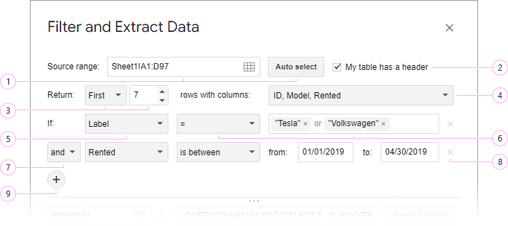
For Filter and Extract Data to work, you should specify your source data table, set up your filter criteria, and decide upon the number of matches to pull:

- Select the range with your source data.
Tip. Pick just one cell within your table and click Auto select. The add-on will instantly highlight all cells with data (till the first blank row & column).
- Alternatively, you can specify the data you want to process by clicking special icons within the Source range field:
- Highlight the cells you need in the sheet and click the Get selection icon to automatically insert the selected range.
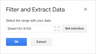
- Click the Select range icon and pick the cells using the dialog box:

To set the range within the dialog box, you can manually type the address, click the rectangle icon to automatically select the entire table, or highlight the necessary cells in the sheet and click the Get selection button.
- If your table columns have titles, tick off the option My table has a header. In this case, the first row will not be matched with your criteria.
- Choose how many rows you'd like to retrieve:
- Pick All to find and pull all matching rows.
- For the tool to look up only a few of the foremost records, click First and enter the number of rows you'd like to see.
- Here you are to decide whether to return matching values from all or only some columns of the range. Check as many individual columns as you need or keep Select all ticked off to get them all.
- And here goes the first condition itself: it starts with If. Its first dropdown lists all search columns of your table. Choose the one that should meet some criterion, e.g. dates that should belong to some period of time or car labels if you need the info on a specific model.
- The second dropdown contains operators that are used in formulas. They signal about different calculation types:
- is empty / is not empty — find blank cells or those with data.
- is error / is not error — find cells that either contain or don't contain any errors.
- = (equals to) — find those cells whose content is exactly the same as the values you specify.
Note. For the add-on to understand your conditions, it provides a special tip on how to enter data correctly. For ease of use, these formats vary based on your spreadsheet locale:
 Tip. When typing the value, press Enter on your keyboard to submit it. This way you can quickly add multiple records to the same condition.
 - ≠ (doesn't equal to) — find those cells whose content is completely different from the values you indicate.
- > (more than) — find cells with numbers that are more than the number you enter.
- >= (more than or equals to) — find cells with numbers that are more than or equal to the number you define.
- < (less than) — find cells with numbers that are less than the number you provide.
- <= (less than or equals to) — find cells with numbers that are less than or equal to your number.
- starts with / ends with — find cells that have the same characters/strings at their beginning or end.
Note. Currently, this operator treats everything as text strings. It wraps your record in double quotes and checks if it occurs in cells. If this doesn't suit your task with numbers, please email us (support@ablebits.com) with a sample and detailed description of your task.
- contains / doesn't contain — find cells that contain or don't contain the records of interest.
Note. Currently, this operator treats everything as text strings. It wraps your record in double quotes and checks if it occurs in cells. If this doesn't suit your task with numbers, please email us (support@ablebits.com) with a sample and detailed description of your task.
- is between — find cells with numbers that are between two numeric values or with dates belonging to a certain period of time.
- This button lets you choose between AND or OR logic for your criteria:

- By default, all additional criteria start with and. This means that all created conditions should be met to get a match.
- If you're okay with either of the criteria to be true for a match, pick the or option from the dropdown instead.
Note. Whatever logic you select, it will be applied to all built conditions. - If you change your mind about any criterion, you can delete it by clicking the Close icon at the end of the criterion line.
- Click on the plus icon to set up more conditions.
Preview and paste the result
Once your requirements are set, you can get the result in a few different ways:

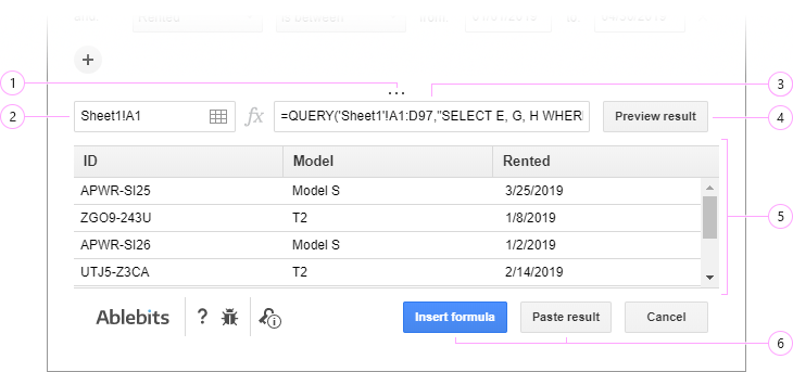
- By clicking on three dots and pulling the border up or down, you can expand or shorten the preview area.
- Based on your conditions, the add-on builds a QUERY formula and shows it to you in this formula field. It filters your data dynamically once anything changes in the original table.
- To take a quick glance at the result before pasting it to your spreadsheet, hit Preview result.
- For the preview, all found matches from the necessary columns will be grouped at the bottom of the Filter and Extract Data window.
Tip. You can tweak your criteria and click Preview result again to get other values.
- Decide where to place the result:
- Use the first dropdown to select the spreadsheet.
- Choose the sheet in the second dropdown.
- In the third field, specify the starting cell (e.g., F12). You can type it manually, select the cell in the sheet and click the Get selection icon, or use the Select range icon to pick the top-left cell for the results.
- Both these buttons insert the result to your spreadsheet but in slightly different ways:
- Click Insert formula to paste everything as the QUERY formula.
- Or have only values returned by choosing Paste result.
Limitations of standard functions used in the formula
Along with our own custom functions, the resulting formula uses a couple of standard ones: QUERY and IMPORTRANGE. Here are some things you should know about the result returned by the formula:
- The first time the destination spreadsheet pulls data from a new source spreadsheet using IMPORTRANGE, it’s necessary to manually allow access permissions.
- If the access rights to the source file are changed, the formula in the result file will start returning a #REF! error.
- IMPORTRANGE has limitations on the number of cells that can be imported. When working with very large spreadsheets, the formula may start to slow down or return errors.
- If there are mixed data types (e.g. numbers and text) within a column, the QUERY function will return only the majority data type leaving the rest as empty cells.
- The QUERY function will automatically skip and not include any completely blank rows from your source data in the final result.
- Due to the way Google Sheets processes formulas, the number of columns in the outcome table is always fixed. If you later add new columns to your source data, they will not automatically appear in the result.
- Google Sheets functions cannot process and take any objects (e.g. images, charts, conditional formatting, etc.) but values to a resulting table.
Please contact us here