Last week we tapped into the insight of Excel logical operators that are used to compare data in different cells. Today, you will see how to extend the use of logical operators and construct more elaborate logical tests to perform more complex calculations and more powerful data analysis. Excel logical functions such as AND, OR, XOR and NOT will help you in doing this. Continue reading
Comments on: Using logical functions in Excel: AND, OR, XOR and NOT
 by Svetlana Cheusheva, updated on
Comments page 3. Total comments: 299
Hello all,
Please help..
Distance 50 kg 100 kg 250 kg 500 kg 1000 kg
Upto 25 NIL NIL NIL NIL NIL
26-100 km 650 750 1000 1150 1500
101-150 km 1000 1250 1500 1750 2000
151-200 km 1250 1500 1750 2000 2250
201-300 km 1500 1750 2000 2500 3000
My query is
If distance 100 km & wg 50 so charge 650/-. if distance 100 km & wg 100 kg charging cost 750/-. if distance 100 km & wg 250 kg charging cost 1000/-. same applicable for 500 kg & 1000 kg.
same for 150 to 300 km & kg 50 to 1000 kg.
my query is condition one is same but condition 2 change so which formula I can use ?
hi Mahesh,
write down your distance on a row on top and quantity in left side colomn such as
100 150 200 250 300 (start this from "B" cell)
50
100
150
200
250
Then apply this in cells and change the value of only 100 in formula with your distance value.
=IF(OR(B18=100,A19=50),650,IF(OR(B18=100,A19=100),750,IF(OR(B18=100,A19=150),850,IF(OR(B18=100,A19=200),900,1000))))
Hi, In my spreadsheet I have the following information:
A2="Gold", B2="Silver" C2="Bronze, D2=a blank field. I'm trying to create a single formula in column E2 which captures the following:
If range A2 to D2 contains "Gold" then E2="Gold";
If range A2 to D2 does not contain "Gold" but it contains "Silver" then E2="Silver";
If range A2 to D2 does not contain "Gold" or "Silver" but contains "Bronze" then E2="Bronze";
If range A2 to D2 fields are all blank fields then E3="unrated"
Hope you can please assist. Thank you.
=IF(OR(A2="Gold",B2="Gold",C2="Gold",D2="Gold"),"Gold",IF(OR(A2"Gold",B2"Gold",C2"Gold",D2"Gold")*OR(A2="Silver",B2="Silver",C2="Silver",D2="Silver"),"Silver",IF(OR(A2"Gold",B2"Gold",C2"Gold",D2"Gold")*OR(A2"Silver",B2"Silver",C2"Silver",D2"Silver")*OR(A2="Bronze",B2="Bronze",C2="Bronze",D2="Bronze"),"Bronze","Unrated")))
May be it will help you
Hi,
I have 2 formulas that both work however I need to have them work together as an "OR" situation and can't come up with the right formula for that. Can you help?
=IF(AND(D45=1,Q45="N"),(I45*0.0925))
=IF(AND(D45=1,Q45="Y"),P45)
HI Dave
do just like this
=IF(AND(D45=1,Q45="N"),(I45*0.0925),IF(AND(D45=1,Q45="Y"),P45),0)
I want to solve simple 3 equation.
Ex:- 6inch> tall, 4 to 6 medium, 4inch<Short.
Hello, Roshan,
try this formula:
=IF(A1>6, "Tall", IF(AND(A1>=4,A1<=6), "Medium", IF(A1<4, "Short", "")))
i am trying to develop a syntax that will allow me to classify patients as having metabolic syndrome. The syndrome satisfies the condition meeting any 3 out of 5 criteria. My data is in excel. truly appreciate for any help.
Thanks, Anam
It's almost impossible to give you a definite formula without any details on the data you use in your table. It would be helpful to know whether the results are numbers or text and which criteria they should meet… What I can do is to only show you a super simplified example of what your data and function may look like
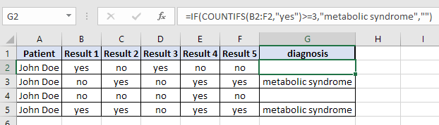
=IF(COUNTIFS(B2:F2,"yes")>=3,"metabolic syndrome","")
COUNTIF counts the number of met criteria, and if it's more than or equal to 3, it returns the result with a diagnosis, otherwise the cell remains empty.
I need help using the IF function, to work out the score range
High =9-13
Moderate =5-8
Low 0-4
Thank you
=IF(AND(A1>=9,A1=5,A1<=8),"Moderate",IF(A1<=4,"Low","")))
Hi, I'm got this formula to work only if it's not blank, but leave the cell blank if there is no number in it,
=IF(T1<=249,"50",IF(T1<=499,"34",IF(T1<=999,"24",IF(T1=2500,"7")))))
I've tried the isblank but to no avail.
Hi Baz,
You can add one more If function that checks for blanks, like this:
=IF(T1="","",IF(T1<=249,50,IF(T1<=499,34,IF(T1<=999,24,IF(T1=2500,7)))))
If cell J1,M1,P1 are = a or p I would like cell B1 and cell C1 = 1
Hi Jim,
Enter the following formula in cells B1 and C1:
=IF(AND(OR($J$1="a",$J$1="p"), OR($M$1="a",$M$1="p"), OR($P$1 ="a",$P$1 ="p")), 1, "")
In Col I Write a formula to give In Col I Write a formula to give rank to student based on below table (Without using IF Condition)
Marks Grades
=33 but less than 60 Pass
>= 60 but less than 70 3rd Div
>=70 but less than 80 2nd Div
>=80 but less than 90 1st Div
>=90 Distinction
rank to student based on below table (Without using IF Condition)
Marks Grades
=33 but less than 60 Pass
>= 60 but less than 70 3rd Div
>=70 but less than 80 2nd Div
>=80 but less than 90 1st Div
>=90 Distinction
plz reply urgent
Use V lookup function
hi trying formula A=B,C=D,E=F,G=H THEN 10000 PLZ HELP
hi hassan,
Just try like this if you need through number format keep numbers in another sheet like this(1,2,3,....10000) give formula, and past below sells it will take automatically up N numbers
=IF(1=2," TRUE "," FALS ")
I need help to write an if statement. i have dates in column E, I need the spreadsheet to add 90 days if answer in column F is yes, and add 365 days if answer in F is NO.
Hi Jessica,
Here's the formula:
=IF(F1="yes", E1+90, IF(F1="no", E1+365, ""))
For scenario 1, I have: =IF(AND(AV2="Y",AD235),AI2," ")
Please help me determine the formula for scenario 3, for AD2 greater than 25 but less than or equal to 35.
Thanks - and not sure why this isn't posting correctly
Our blog engine often mangles "<" and ">" characters in formulas, sorry for this. You can specify all 3 conditions in the AND statement, like this:
=IF(AND(AV2="Y", AD2>25, AD2<=35), AI2,"")
I have to make 3 calculations based on two factors:
1. If a variable 1 (AV) is “Y” and the second variable (AD) is less than or equal to X, then input the third variable (AI) or leave blank.
2. If a variable 1 (AV) is “Y” and the second variable is greater than X, then input the third variable (AI) or leave blank.
3. If a variable 1 (AV) is “Y” and the second variable is greater than X, then input the third variable (AI) or leave blank. I need to calculate for AD2 between 25 and 35 (25<AD2<=35)
For scenario 1, I have: =IF(AND(AV2="Y",AD235),AI2," ")
Please help me determine the formula for scenario 3.
Thanks
Hi!
If you want to handle all 3 scenarios with a single formula, then you have to use nested IFs. To be able to suggest an exact formula, I need to know the actual values for all 3 scenarios because this determines the order of nested IF's.
Hi Amanda,
I want to ask you,How we use AND or OR logical function with IF condition?
Please Help with atleast two example.
Hello!
Check out the following examples:
Excel IF function with multiple AND/OR conditions
Hi,
Here's one for you:
I've got a column containing the following values: "1", "2", "3", and "-".
I want to nested If/OR formula to return the follow.
If Column A contains a "1", return a 1
If Column A contains a "2", return a 0
If Column A contains a "-" OR "3", return a 'FALSE'
What's the best formula?
Hi Liz,
Try this one:
=IF(A1=1, 1, IF(A1=2, 0, IF(OR(A1=3, A1="-"), FALSE, "")))
I want to use If formula. Generally we do =if(A2>4, "YES", "No") and i want to use =If(A2>4, "B2", "") but is not working. Any idea for do this formula.
I done it from help by your above comments. Thank You.
PLEASE HOW DO I CREATE THIS FORMULAR. FOR EXAMPLE, IF A3 > B2, SUBTRACT B2 FROM A3 AND IF IT IS REVERSE AS IN IF B2 >A3 , SUBTRACT A3 FROM B2.
Hi Jolly,
Here you go:
=IF(A3>B2, A3-B2, B2-A3)
=IF(AND(E12>0,"Closed","Open"), OR (B12>0,"Open".""))
What's wrong with my formula
I'm trying to say if E12 has no date(there is a reference formula in it so I used E12>0) then it equals blank being "", but if it has a date in it, it is open.
Then if B12 has no date it is open, but if B12 has a date, it is closed. B12 also has a reference formula in it.
Are these two different formulas you need or one?
=if(e12=0," ","Open")
=if(b12=0,"Open","Closed")
Your 2nd formula has a period instead of a comma.
Hi, I'm trying to find a way of achieving the following,
if A1 has a text entry of "W" then add 1 to cell B5, if A2 has a text entry of "L" then add 0 to C5. These have to be interchangeable so if A1 has a "L" entry enter 0 to B5, and if A2 is "W" add 1 to C5
Hello Graham,
You can use the following formulas.
For B5:=IF(A1="W", 1, IF(A1="L", 0, ""))
For C5:=IF(A2="W", 1, IF(A2="L", 0, ""))
I have 3 columns
A: has member ID
B: Date
C: Trainer ID
I want to highlight members who saw different trainers on the same day..
Will this work?
=IF(XOR(AND((A3=A2),(B3=B2)),(C3=C2)),0,1)
Appreciate your help
Hi Asiya,
Try the following formula:
=IF(COUNTIFS(A:A,A1,B:B,B1,C:C,C1)>1, IF(COUNTIFS(A:A,A1,B:B,B1) - COUNTIFS(A:A,A1,B:B,B1,C:C,C1) = 0,"not different", "different"),IF(COUNTIFS(A:A,A1,B:B,B1)>1,"different","not different"))
I have a cell (A1) that can contain the values of 6, 12 or 18.
If A1 is 6, I want cell B2 to show 0; if A1 is 12, I want cell B2 to show 12; if A1 is 18, I want cell B2 to show 18.
I've tried various combinations using IF and OR but can't arrive at the desired conclusion. Can you help?
Hello Uncle Dave,
Try the following formula:
=IF(A1=6, 0, A1)
Hi,
working on an excel with a lot of tabs.
I need a sum, that checks different values, and sums them if all of them are true. Only the last part of the formula should check, if either one of the two conditions are true.
Currently I am working with Sumifs, that works pretty good, except for the last part, where it should only sum, if one of the two values is true.
This is the formula:
=SUMIFS(Export!$D:$D;Export!$G:$G;B$17;Export!$Z:$Z;"2016-11-*";Export!$H:$H;"Forecast*";Export!$K:$K;"Open";Export!$AH:$AH;"*Medium*";Export!$AI:$AI;"*Medium*")
So basically it should sum the values, if "Medium" is mentioned in the column AH AND/OR AI .
Thank you very much for your help.
Hi Jean-Luc,
Try the following formula:
= SUMIFS(Export!$D:$D;Export!$G:$G;B$17;Export!$Z:$Z;"2016-11-*";Export!$H:$H;"Forecast*";Export!$K:$K;"Open";Export!$AH:$AH;"*Medium*") + SUMIFS(Export!$D:$D;Export!$G:$G;B$17;Export!$Z:$Z;"2016-11-*";Export!$H:$H;"Forecast*";Export!$K:$K;"Open";Export!$AI:$AI;"*Medium*") - SUMIFS(Export!$D:$D;Export!$G:$G;B$17;Export!$Z:$Z;"2016-11-*";Export!$H:$H;"Forecast*";Export!$K:$K;"Open";Export!$AH:$AH;"*Medium*";Export!$AI:$AI;"*Medium*")
IF SALARY >= 5565.61 THEN SALARY X 12.5%
IF SALARY >= 3566.05 OR SALARY =1783.84 OR SALARY <=3566.04 THEN SALARY X 17.5%
IF SALARAY <=1783.83 THEN SALARY X 20%
How i write this in excel? need help
IF SALARY >= 5565.61 THEN SALARY X 12.5%
IF SALARY >= 3566.05 OR SALARY =1783.84 OR SALARY <=3566.04 THEN SALARY X 17.5%
IF SALARAY <=1783.83 THEN SALARY X 20%
Hi Svetlana,
Need your help in calculating the following problem
Volume Product Type
200 A
300 B
200 C
200 A
100 B
All the product type columns are selected via drop down list using data validation option in excel. My problem is that i need to sum up each product type separately.So can you help me out in this..
Hi Shash,
Please use Pivot Tables to solve your task.
Hi Svetlana,
I need help to solve the following problem.
Cells
A B C D E
1 Yes Yes Yes Yes Yes
2 Yes Yes Yes No No
3 No No No No No
4 Yes Yes Yes
Svetlana,
If all cells in Row 1 = Yes then response is Yes in cell E1
If any cell in Row 2 = No then response is No in cell E2
If all cells in Row 3 = No then the response is No in cell E3
If any cell in Row 4 has a blank then response in E4 is blank, empty.
Hope you can help with a formula.
Hi Henry,
Try the following formula:
=IF(COUNTIF($A1:$E1, "")>0, "blank", IF(COUNTIF($A1:$E1, "yes")=5, "yes", "no"))
"=IF(AND(A2="White",B21),15,IF(AND(A2="Not white",B21),12,0))))"
=IF(AND(A2="White",B21),15,IF(AND(A2="Not white",B21),12,0))))
Hello Svetlana,
*Something went wrong in my previous question. Here's the correct question.
I have been trying to crack this for quite a while now. Your help will be much appreciated.
I am trying to achieve the following rate/pc:
If color is white and pcs is less than or equal to 1, rate/pc = 10
If color is white and pcs is greater than 1, rate/pc = 5
If color is not white and pcs is less than or equal to 1, rate/pc = 15
If color is not white and pcs is greater than 1, rate/pc = 12
I have been able to get the first 3 conditions correct using if(and) and if(not) however I can't get the 4th condition to work. Is there a formula for 2 not conditions?
I look forward to hearing from you soon. Thanks in advance.
=IF(AND(A2="White",B21),15,IF(AND(A2="Not white",B21),12,0))))
Help in Excel formula that is If sheet 1 cell C2 are equal or greater than 21 then copy data sheet 1 cell A2 to C2 and paste in Sheet 2 A2 to C2 if not equal 21 then do not copy data
Hello Nisar,
Enter the following formula in Sheet2 A2, and then drag it rightwards up to cell C2:
=IF(Sheet1!$C$2>=21, Sheet1!A2, "")
i AM HIGHLY THANK FULL FORMULLA WORKS
A1 B1 C1 D1 E1 F1 D1
_________________________________________________
1450 1440 1073 301 66 73 D2
HOW I USE FUNCTION IN G2 CELL IN ABOUT CONSTANT B1 WHEN F1 IS GREATER THAN EQUAL TO E1
OTHER WISE MINUS E1 FROM B1 WHEN E1 IS GREATER THAN F1
Hello LAXMIDHAR,
If my understanding of your task is correct, you can use the following formula:
=IF(F1>=E1, B1, B1-E1)
hi, can anyone help me?
I don't to write like this
=IF(A1=10,F1=0,IF(A1=12,F1=0,IF(A1=13,F1=0,IF(A1=16,F1=0,IF(A1=18,F1=0,IF(A1=90,F1=0,IF(A1=91,F1=0,IF(A1=92,F1=0,IF(A1=93,F1=0,10000)))))))))
I want a shorter
Hi!
You can use the OR function instead of nested If's:
=IF(OR(A1=10, A1=12, A1=13, A1=16, A1=18, A1=90, A1=91, A1=92, A1=93), 0, 10000)
Hello! Good evening.
Pls guide me solve the problem.
1- If Table A1 value is 1, B1 is 54,
2- In continuously If A2 value is 0, b2 value is 0.
then whats the formula apply to get the total no. of receipts in both tables C1,C2. Pls give the one formula for both tables.
Recpt. No.
From To Total
1 54 ?
0 0 ?
Hello, Prem,
For us to be able to assist you better, please give us the result you need in C1 and C2.
Can you help me with this? If A1:B1 match any A:B then add matching C cells?
Hello, TJ,
Please try this formula:
=IF(AND(INDIRECT("A1")=A3,INDIRECT("B1")=B3),"Matching","Non-matching")
A1 = RECEIVED / CANCELLED / DECLINED (Dropdown)
If A1="CANCELLED" then A2, A3, A4... will show CANCELLED
If A1="DECLINED" then A2, A3, A4... will show DECLINED
but
If A1="RECEIVED" then A2, A3, A4... must be blank
Please advise. Thank you
GOTCHA! :D
Hi, I am lost. can you help me with this problem.
I want to choose from a drop down list for the following
1) choose either ATM or CDM
2) choose either Shift1 or Shift2
3) choose the units available example 100, 200, 300 etc
4) choosing from 1) and 2) and 3) will get the result
the result will show
ATM Shift1 100 units = xxx
ATM Shift1 200 units = yyy
ATM Shift1 300 units = zzz
CDM Shift1 100 units = aaa
CDM Shift1 200 units = bbb
CDM Shift1 300 units = ccc
ATM Shift2 100 units = ddd
and so on
Is it possible? Please advise. Thanks
Hello, Michelle,
You can read how to create a dropdown for a worksheet in Making a cascading (dependent) Excel drop down list. For us to be able to assist you better, please describe the condition for the expected result.
Hi
I have a 3 in one if statement to put value to certain conditions:
=IF(AND(C26>=0,C26=3,C26=5,5,"error")))))
If I make the last condition = 5, it gives me the "error" msg for anything else typed in - which is correct. When I say >5 it gives me 5 for any word typed in which should be giving me "error" msg? How do I fix this?
Thank you.
Hello, Shirleen,
This formula isn't true since a value cannot be equal to 3 and 5.5 at the same time. We suppose that you need a formula like this:
=IF(OR(C26>=0,C26=3,C26=5.5),"error", "")
Hi Svetlana
When all the cells are blank. As the cells are filled "pass"/"fail", then filled appropriately.
Thanks
Hi Phil ,
Then you can add one more AND function that checks for blank cells:
=IF(AND(D45="", D46="", D47="", D48=""), "", IF(AND(D45="Pass", D46="Pass", D47="Pass", D48="Pass"), "Pass", "Fail"))
Alternatively, you can use COUNTIF to make the formula more compact:
=IF(COUNTIF(D45:D48, "")=4, "", IF(COUNTIF(D45:D48, "pass")=4, "Pass", "Fail"))
Hi
I have a column of cells in which "pass" or "fail" is entered. I have a formula in the last cell (D49) set to auto fill, as an overall "fail" if only one of the cells has "fail" in it.
=IF((AND(D45="Pass", D46="Pass", D47="Pass", D48="Pass")), "Pass", "Fail")
This is what I want. However, when the other cells are blank, it auto fills to "fail", as no "pass" is present. I would like D49 to be blank if there is no text in the Cells D45 to D46. What can I add to the formula to keep it blank if cells D45 to D48 are blank?
Thanks
Hi Phil,
Do you want D49 to be blank when all the cells (D45 to D48) are blank or when at least one cell is blank?
HI i need help. im trying to ask excel to evaluate a less than but greater than scenario. for example: IF(A3 is greater than 1 but less than 100) , "...." ... Anybody?
Hi Francisco,
You can use an AND statement, like this:
=IF(AND(A3>1, A3<100), value_if_true, value_if_false)
formula in O4 cell D4-(C4+F4+I4+L4) and second formula IF(O4>=0,0,IF(O4<=0,O4)). how to used both formula in same cell.
Hello PANKAJ,
If you want to perform all the calculations with a single formula, here you go:
=IF(D4-(C4+F4+I4+L4)>=0, 0, D4-(C4+F4+I4+L4))
If you are looking for something different, please clarify.
Please send me few excel work sheet for office usage, & practise please it my request for you....
please
Hi,
I am trying to determine how i can take the value of two different cells and return the difference in another cell. I realize that if I subtract one cell from the other it will give me the difference. However this will not work correctly if the first cell's value is less then the 2nd cells value. I need the third cell to show either a positive or negative number based on the values entered into the first two cells.
Thank You
Hi Ron,
I am not sure I understand the problem. For example, if A1 is 1 and B1 is 3, and you put the formula A1-B1 in C1, the answer will be -2.
If you want the formula to do something different, please clarify.
Hi,
I'm looking for a formula that will count. EG if both cells a1 and b1 are negative #s, then enter cell b1 in cell c1.
Hi Crystal,
If #s means negative numbers, you can enter the following formula in C1:
=IF(AND(A1<0, B1<0), B1, "")
i want to give 3logics by using IF condition i.e.,if a1 is greater than30=ok,lessthan30=Not good and if respective cell contain negative figure =NA, then how to give formula
Hello KRISHNA,
You can use a nested IF formula like this:
=IF(A2<0, "NA", IF(A2<30, "not good", "ok"))
thank You
Hi
i am trying to work out a formula were a cell have 3 drop down suggestions, from the dropdown picked i want another cell to be able to determin my anser
=IF(AB5="introduced",AE5*0.2),IF(AB5="introduced returning","5"),IF(AB5="existing","0")
thought this might work but i am getting "value" returning and not the answer i need
Kind regards
Hi Ken,
The correct syntax of a nested IF formula is as follows:
=IF(AB5="introduced",AE5*0.2, IF(AB5="introduced returning", 5, IF(AB5="existing", 0)))
Thank you very much.. silly mistake on my part , works perfect.
I ma trying to put if and but to get the answer to be a number of a difference between two cells how can i take this up , the results are coming as just =A1-B1 , How do i get the formula to return the result of this =IF(AND(EV6>0,EV6<=B6),"=EV3-B3","0")
Thanks
Here you go:
=IF(AND(EV6>0,EV6<=B6), EV3-B3, 0)
Hi I am having trouble creating a formula to reflect:
If preferred is True (F4), or the budget (C4) amount is greater than the quote (D4), then display the quote (D4) less the discount (H4), otherwise display nothing.
My formula: =IF((F4="true")*OR(C4>=D4-H4),D4-H4,"")
is not showing all the necessary information. Would really appreciate the help.
Thank you
Hi Kelly,
Here is th correct syntax if F4 is the Boolean value TRUE:
=IF(OR(F4=TRUE, C4>=D4-H4),D4-H4,"")
If F4 is a text value:
=IF(OR(F4="true", C4>=D4-H4),D4-H4,"")
=IF(AND(OR(A2=1.5, A2=3.5,A2=4,A2=51,A2=54), B2<10),"Excluded",""))
I want to add formula if A2 is 1.5/3.5/4/51/54 and B2<10, then C2 should be displayed with value "Excluded"
Hi Deepa,
Your formula is correct except for an extra closing parenthesis at the end:
=IF(AND(OR(A2=1.5,A2=3.5,A2=4,A2=51,A2=54),B2<10),"Excluded","")
Hi I Need Help
I am making some test reports ,I have given three grades for each parameter like deficient, optimum, excess.
we have given formula for three conditions, there forma-ls =IF( H37 50,"Excess",".")
my problem is how i can insert these three logical function in one Cell
please Help
Hi Prasad,
You can use nested IF's like in the following example:
https://www.ablebits.com/office-addins-blog/nested-if-excel-multiple-conditions/
I'm trying to input a formula where
Column R7 has pricing where some rows are € and some are $. I want to inpit a formula on the next column that if it contains the $ price - so basically if € price is in R7 it needs to be multiplied by 1.1, if $ price it should just be price given - make sense?
Hi Simone,
Are these text values with the 1st character being either € or $, or are they numbers with the Currency format applied?
The cell selection is number then Accounting. In the upper bar you only see the numeric value.
hi please me
i struck on a formula.
suppose A=A then A*100 but not > 200
Sorry Gopal, your conditions are not clear. Could you try to explain diferently? For example:
If A1="text" or X value,
then A1*100,
otherwise what?
can you help me with the following grading system
80%-100% A
70-79% B2
65-69% B3
60-64% C4
55-59% C5
50-54% C6
45-49% D7
40-44% E8
below 40 F9
I can help you if you want to learn
Hi EMMANUEL,
You can use nested IF functions like in the following example:
https://www.ablebits.com/office-addins-blog/nested-if-excel-multiple-conditions/