Combine duplicate rows in Google Sheets
When the same records take several lines, the Combine Duplicate Rows add-on is your best assistant for bringing all relevant information together. This page shows how to combine rows with duplicate entries that have unique information in adjacent columns in 3 simple steps.

Video: How to combine duplicate rows in Google Sheets
Before you start
Formulas
The add-on processes values only. There is no technical possibility for it to keep your formulas when it combines data from several rows into one.
Merged cells
The add-on doesn't process merged cells. If there are any in the rows you want to combine, they will be unmerged, and only the value from the top-left cell will be kept.
Backup copies
We care about your data and suggest you always create backup copies of your spreadsheets. A special option of the add-on will do that for you if you select it.
How to use the Combine Duplicate Rows tool
Start Combine Duplicate Rows
Go to Extensions > Remove Duplicates > Combine duplicate rows to run the add-on:

Step 1: Select your data
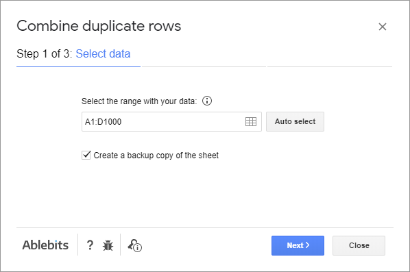
Here you are to adjust the range where you want to combine duplicated rows:

- The add-on picks the used range — cells with data till the blank row & column — by default. To modify it, enter the needed address in the field manually.
- Click the Get selection icon to automatically insert the range that is currently selected in your spreadsheet into the field.
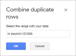
- Click the Select range icon to open a dialog box:

The dialog box allows you to pick your data in different ways:
- Enter the range in the Select the range with your data field using your keyboard.
- Pick a cell in the table and click the rectangle icon to select the entire table (up to the first empty row and column).
- Highlight the necessary cells and click the Get selection button to auto-insert the range.
Select the necessary cells and click OK to confirm the reference.
- Use the Auto select button to detect the used range (till the first blank row and column) with your data automatically.
- We always recommend ticking off the option to Create a backup copy of the sheet. It will duplicate the original spreadsheet before its records are combined.
Note. Make the copy of your sheet especially if there are any formulas in the range.
Click Next to continue to step 2.
Step 2: Identify key columns
This step lets you define the columns with duplicate key values that you want to combine:

- You will see three additional options here:
- Data has header row. If you have a title row in the selection, choose this option to see column names and leave the top row intact.
- Skip empty cells. If there are blanks in your key column, you can leave them as they are. Otherwise, the add-on will join them into one row as well.
- Match case. Select this option if you want to consider such records as A1 and a1 as different. Leave this option unchecked to ignore the case of the key values and combine A1 and a1 into one row.
- To use many matching columns, use the checkbox at the top of the table to tick off them all at once.
Note. Make sure to leave out the columns with the unique entries to merge. You will specify how to combine the values in adjacent columns on step 3.
- Choose columns with the key values to combine from the list. It can be one column, e.g. a column with IDs, or a combination of columns like first and last names. In our example, it will bring together only those rows that have the same first name J.K. and last name Rowling.
Note. The add-on will look for matches in all the columns of interest at once. It doesn't matter if the records are not directly one under the other, the tool will combine them anyway, so you can keep your current sorting order.
Once you specify key columns on this step, click Next to follow to the last step.
Or choose Back to change the range with data.
Step 3: Choose columns with the values to merge
The last step lets you identify the values to merge in your selection along with the way to do it:

- There are three additional options that refer to the merge process:
- Delete duplicate values. This will let you keep only unique records.
For example, if you are combining rows by order IDs and merging names, one ID may take several rows with the same name. You can keep the first occurrence of the name in the resulting row and avoid repetitions.
 Note. This option does not apply to columns with numbers you choose to calculate.
 - Skip empty cells. Select this option to avoid adding extra delimiters for empty cells. Disregard this if it's important for you to see the blanks.
- If all your columns contain data of the same type, use the Synchronize action option to match the way of merging them. Once you set up the way to merge records in one column, it will be auto-set for all other selected columns.
- Delete duplicate values. This will let you keep only unique records.
- Use the top checkbox to select all columns.
Note. For the columns you don't select here, not only won't their values be merged, but also only the first record for each key value will remain. Other records will be lost.Tip. Combine this option with Synchronize action to set the way to merge for all columns at once.
- For each column of interest, use the Action and Delimiter / function areas to decide on the way to process the data:
- Select Merge values if you want to list all entries that refer to the same record.
Pick one of standard delimiters (Line break, Semicolon, Comma, Space) from the drop-down list or enter any custom separators in the same field. For example, you can bring all book titles to the same cell and use a line break to separate them within a cell:

-
Choose to Calculate numbers and select the function to apply when you want to subtotal the numbers that refer to the same record:
 Tip. Even though the name of the action implies working with numbers, you can use the COUNTA function for text values, e.g. count the number of ordered products instead of listing their names.
- Select Merge values if you want to list all entries that refer to the same record.
Get the result
Once you set up the action for all columns with the values you'd like to keep, click Finish and see the summary of the merged rows in the add-on window:

How to work with scenarios
If Combine Duplicate Rows is your go-to add-on, chances are you run it often and go through the same options over again. To help you automate the process a bit, we implemented scenarios for this tool.
What is a scenario
A scenario is a set of all options that you choose on each step of the add-on. You can save these settings to run later either on the same table with new data or on another table of the same structure.
Save the scenario
When the add-on finishes combining duplicate rows and shows you the result message, click Save scenario:

You will see a short summary of all options you have used just now — this is your scenario preview:

- Name your scenario so you could understand what it does and quickly find it among other scenarios.
- Select the sheet that you want to alter with this scenario:
- To process a sheet where your mouse cursor stands when you run the scenario, choose [Selected sheet].
- Or pick any particular sheet to always handle it no matter where you stand in the spreadsheet when you start the scenario.
- Set the range that you want to alter with the scenario:
- Choose [Selected range] and the scenario will be applied to cells that are selected at the moment.
- Pick [All data] to have the add-on detect the entire used range.
- Or specify a particular range to process.
- Look through the options you're about to save to make sure everything is correct:
 Note. These settings cannot be modified here. If you want to adjust some of them, you will need to restart the add-on and fine-tune the options while going through the steps.
If everything looks good, click Save.
Run your scenario
To start the scenario, go to Extensions > Remove Duplicates > Scenarios, select the required scenario and click Start.

Combine Duplicate Rows will begin to work with the data according to the scenario settings.
Once it's done, you will get the result message saying what scenario has just worked and what it's processed:

Edit or delete scenarios
To view the scenario or to change the sheet and the range you want to alter, go to the same Extensions > Remove Duplicates > Scenarios menu, pick the scenario and select Edit this time:

You will see the entire scenario outline again:

You can give it a new name and select other sheet & range.
If you make any changes, press Save to keep them. Click Run to start the scenario right away, or hit Delete to remove it completely.
Share scenarios
You can easily export one or more scenarios and share them with your teammates or sync across your different Google accounts.
Share a single scenario
To share a single scenario, go to Extensions > Remove Duplicates > Scenarios > desired scenario > Export & share:

You’ll be prompted to save the scenario on your computer:

Click Save, and your browser will prompt you to pick a location to store the file. Once the file is saved, close the add-on window.
You can now share the file with anyone using Combine Duplicate Rows, and they’ll be able to import the scenario directly.
Share all scenarios
To export all the scenarios you’ve created, navigate to Extensions > Remove Duplicates > Scenarios, then select Export & share all scenarios:

The add-on will notify you that all scenarios will be saved to your computer:

Click Save, and your browser will open a window to specify the save location. After saving, you can close the add-on window.
Now you can send this file to other people using Combine Duplicate Rows, and they’ll be able to import all the scenarios into their tool.
Import scenarios
To bring in scenarios shared with you, go to Remove Duplicates > Scenarios > Import scenarios:

The add-on will ask you to choose the file with the saved scenarios. Click Browse:

After importing, a message will display the number of scenarios successfully added:

Tip. The tool imports all scenarios from the file by default. If conflicts occur with your already existing scenarios, you’ll be notified.
You’ll find all imported scenarios under Remove Duplicates > Scenarios, ready to be used or modified:

Please contact us here