Combine Rows in Excel

With Text Toolkit for Microsoft Excel

Combine Rows is an easy-to-use tool for merging rows by duplicates in key columns. It's part of Text Toolkit for Excel.

Start Combine Rows

To start your work with the Combine Rows tool, click the Text Toolkit icon on the Home tab in your Excel:
This is the Text Toolkit icon.
At the bottom of the Text Toolkit pane, find the Combine Rows icon. Click it to proceed:

Run the Combine Rows tool.

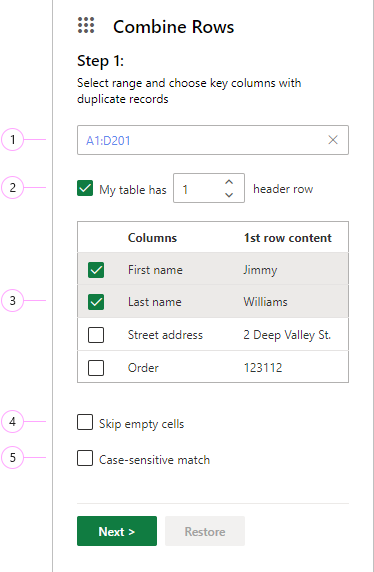
Step 1: Select the range and specify key columns

Decide on your range and key columns.

  1. Select a range containing the rows you would like to combine. It should consist of at least two columns and two rows.
  2. If there are header rows in your table, specify how many. Please note that header rows won't be processed.
  3. Check columns where the add-in will look for duplicates, i.e. key columns.
  4. If blank cells in key columns need to be ignored, select the Skip empty cells option.
  5. To take letter case into account, opt for Case-sensitive match.

Click Next.

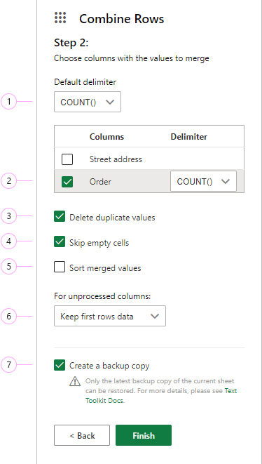
Step 2: Choose merge settings

Decide on merge settings.

  1. Use this drop-down list to choose a default delimiter or a function for the values that are going to be merged.

    You can pick one of the preset delimiters: a space, a comma, a semicolon, a period, or a line break.
    Pick a delimiter.

    You can also use another delimiter if you want to. Simply type it into the field.

    A list of previously used delimiters is under History:
    Here you can see a list of previously used delimiters.

    The functions available are as follows: AVERAGE, COUNT, COUNTA, MAX, MIN, SUM, STDEV.P, STDEV.S, and PRODUCT.
    Here is the list of functions to choose from.

  2. Select columns containing the values to be merged. Change the default delimiter (or function) to another one if needed.
    Note. If you want to return to the default delimiter (or function) after choosing another one for any of your columns, clear the checkbox next to the column of interest and select this column once again.
  3. To dedupe the resulting data, check the Delete duplicate values option.
  4. Opt for Skip empty cells to exclude blanks from the results.
  5. If the resulting strings should be arranged in alphabetical or numerical order, select Sort merged values.
  6. Decide what values to display in the other columns and pick the corresponding option:
    Decide which row to show for unprocessed columns.
  7. With the Create a backup copy option selected, the Restore button is added (you can see it in step 1 of the tool), and a hidden copy of your sheet will be saved. After the tool has processed your data, the Restore button gets enabled. You can click it and return to the previous version of the processed sheet if necessary.
    Here's the Restore button.

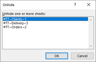
    Tip. To see available backup copies, right-click any sheet tab in your Excel workbook and choose "Unhide".

    Unhide any of the backup sheets that you can see in the list.

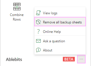
    Note. You can delete hidden backups with the Remove all backup sheets option in the More menu. To see it, click the three dots in the lower-right corner of the Text Toolkit pane:

    Find the Remove all backup sheets option in the More menu.

As soon as you choose the necessary settings, click Finish.

Post a comment

Seen by everyone, do not publish license keys and sensitive personal info!

If you have any questions or issues with this add-in, please feel free to post your concerns in the comments area. As soon as we answer, a notification message will be sent to your e-mail. If you do not want to share your thoughts in public, please contact us at support@ablebits.com.