Combine data from multiple sheets into one
This tutorial shows how to use the Combine Sheets add-on to join tables from multiple sheets together. Learn how to save the column order and initial formatting of combined tables and put the result where you decide. Have the united data pasted as values or get it as a formula to reflect all future changes made in the original sheets.

Video: How to pull data from other Google sheets into one table
Before you start
Please bear in mind that Google Sheets limits the total number of possible cells in your file up to 10 million cells.
How to use the Combine Sheets add-on
Start Combine Sheets
Run the add-on from the Google Sheets menu: Extensions > Combine Sheets > Start:

Step 1: Select the sheets to combine
On this step, you choose the spreadsheets you want to combine:

- Tick off the Sheets checkbox if you want to combine all spreadsheets from the tree view together.
- Use this triangle next to the file name to expand/collapse the list of all sheets from this spreadsheet. Select the sheets you want to combine.
Tip. If you plan to combine using a formula and want to select some blank sheets where the data may appear later, make sure these sheets have the same header row as in other sheets. Otherwise, the formula won't be able to include such sheets in the result.
As for the range for such sheets, don't specify it (like A1:F1). Instead, keep it as All data, and the add-on will do the rest. - Press Add files from Drive to import and merge more files.
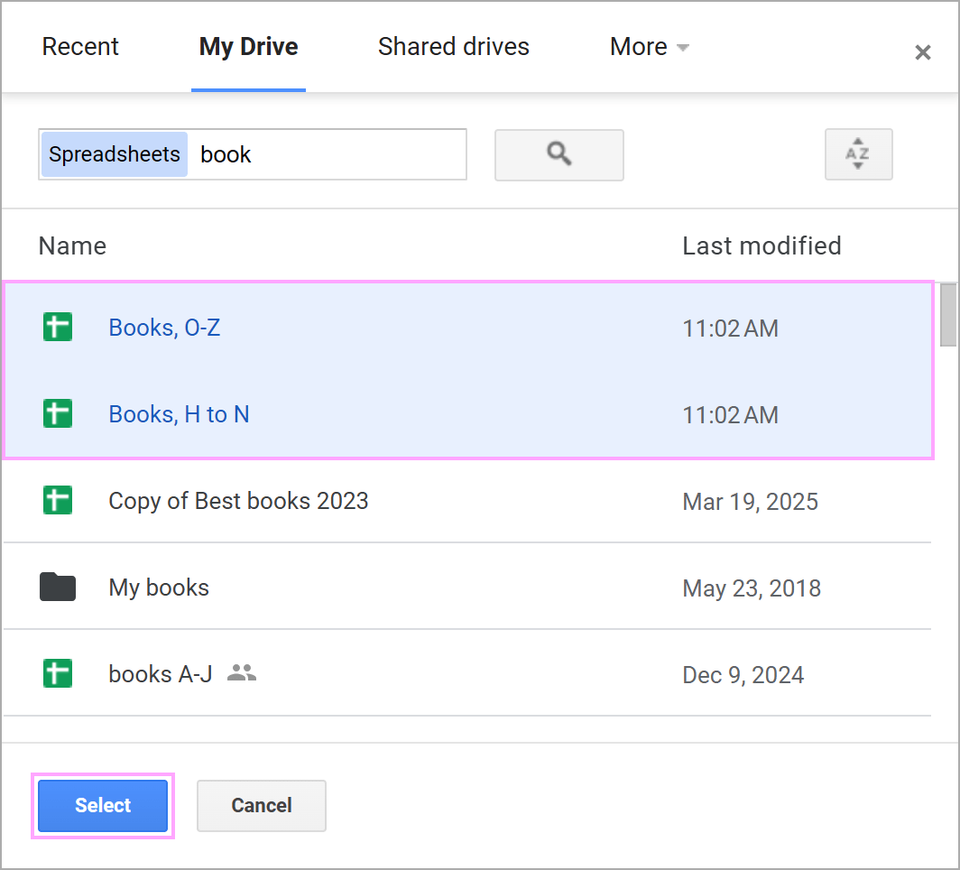
Tip. If you don't remember the exact location of the file or simply don't want to browse from folder to folder, use the Search field at the top of the window instead.
Before the search, feel free to stay on the Recent tab to look through all recently opened spreadsheets, or switch to a specific tab to search the specific place: My Drive, Shared drives, Shared with me, or Starred.

Then simply enter the word your spreadsheet name may contain and press Search.

The add-on will scan the selected Drive folder for both exact and partial name matches.
Tip. You can add a few files at a time. Keep the Ctrl button pressed and click the sheets names to see them highlighted in light-blue. Click Select to work with these files or click on the names once again to cancel the choice:
- If you added the spreadsheet by mistake or simply no longer want to use it for merging, select it in the list and click the Exclude button.
- If some sheets have extra data, you can limit the range of interest. To do that, click All data next to the sheet name under the Ranges column and do one of the following:
- Type the range.
- Click the Select range icon and highlight the cells on the sheet manually.
- Click the Select range icon, select any cell within your table, and press Auto select. This will automatically pick the used range — till the first empty column & row:

When the sheets you want to work with are selected, click Next.
Step 2: Select the columns to combine
Decide which columns from your tables should be combined at this stage:

- If your tables contain similar columns arranged in different ways, pick Consider table headers. This option lets the add-on combine worksheets based on their headers.
Tip. This way, you will avoid extra header rows before each table — only the data will be transferred.
- Select the top checkbox to include all columns in the result, or check the boxes next to specific columns to combine only them.
- Sheets with column indicates how many sheets you chose to combine contain each column. This way, you'll know if any sheet lacks this or that column.
- If the column list is too long, you can double-check the number of the selected columns here.
Step 3: Tweak extra options to combine spreadsheets into one
The add-on lets you personalize the way it's going to combine data:

- Choose how to copy the data from the sheets
- Add sheet names in a new column to the right will insert a new column with the names of the original sheets next to the combined data. This will help you easily identify which sheet each row of data came from.
- Use a formula to combine sheets. This one will pull data using a specially created formula. The formula will auto-update records whenever they change in source sheets or if the number of rows and/or columns changes in original tables.
Note. There are some peculiarities in the way formula combines data. We strongly suggest you go through them to understand what exactly you can expect from the formula.
- If you want to save the original look of each table, check the box called Preserve formatting.
- The last option, Separate the copied ranges by, will add either an empty row or the name of the source sheet between the tables so you could easily find where one range ends and the next one begins.
- Optionally sort the result by one or several columns either A>Z or Z>A. Click that plus icon to add more columns to sort by.
- Decide where to put the result:
- Select New spreadsheet to get the resulting table in a new file. Combine Sheets will create it automatically in your Drive. Click Browse to change the location and pick a destination folder for a new file on your Drive.
Note. In Combine Sheets within Power Tools, you can also manually enter the path to the destination folder.
- Use the New sheet option to place your output table to a new tab within the opened file.
- Next is the possibility to add more sheets to the existing result. Select that resulting sheet in this drop-down (assuming the add-on is opened from the spreadsheet with the result). All sheets selected on Step 1 will then be added to this resulting table.
Tip. Look through the detailed instructions on how to add sheets to the existing result below.
- Select New spreadsheet to get the resulting table in a new file. Combine Sheets will create it automatically in your Drive. Click Browse to change the location and pick a destination folder for a new file on your Drive.
- In case you want to put the combined data to a particular place in a current spreadsheet, go with Custom location and enter or select the leftmost cell of the future joined table.
Get the result
As the final confirmation, you will see the message saying how many sheets have been combined. Your data will be collected together in a new place according to the options you selected.

Combine several files with a formula
When you combine data from different files and choose to have the result as a formula, the add-on uses standard Google Sheets IMPORTRANGE to pull records together.
By default, for the function to work properly, you must grant it permissions to connect to other spreadsheets. Otherwise, you will see formula errors rather than the combined data.
Our add-on suggests the way of doing that correctly. See how to do that in the following video or read the instructions below.
Video: Enable the formula built by Combine Sheets
- Whenever IMPORTRANGE is used in the outcome formula, you will see a resulting message telling you how to connect the function to other files:

- For your convenience, the add-on creates two sheets:
- Combined data with your outcome formula.
- Connect files to IMPORTRANGE where you are to grant all permissions.
Tip. If you place the result to a new spreadsheet, click the Open new spreadsheet link to jump right to the Connect files tab. Run Combine Sheets first to enable our custom formula, then proceed with the steps below.
If you place the result to the current file, the Connect files sheet will become active automatically. - The Connect files tab will always contain the following:
- the description of how to connect the sheets
- the reminder to run Combine Sheets (which is unnecessary unless you put the result to a new spreadsheet where our own custom function must be enabled as well)
- the list of all spreadsheets that must be accessed by the formula
- the access status
Just hover your mouse over the errors in the Access status column and press each Allow access button that will appear:

- As soon as you do that, the Access status will say Connected and the cells will turn green:

Once all spreadsheets are connected, go to the Combined data tab and wait a bit till the result is loaded.
Limitations of standard functions used in the formula
Along with our own custom functions, the resulting formula uses a couple of standard ones: QUERY and IMPORTRANGE. Here are some things you should know about the result returned by the formula:
- If you place the formula to a new spreadsheet, our custom functions (COLUMN_LIST_CS, CONSIDER_HEADERS_CS) won't start working until you run Combine Sheets once. Since that file is newly created, this way you enable our custom function there.Do that before granting the IMPORTRANGE access and you won't have to reload the spreadsheet as well.
- Formulas won't work without our add-on. Whether you use the tool to create formulas or make copies of the shared files with formulas, you should have the add-on installed. Otherwise, there's just nothing to maintain our custom functions.
- The QUERY function from the outcome formula doesn't include completely blank rows to the result.
- If there are mixed data types (e.g. numbers and text) within a column, the QUERY function will return only the majority data type leaving the rest as empty cells.
- If some columns are missing from one or more tables, as a result, you would normally expect to see empty cells in such columns:

However, QUERY makes us place strings of spaces into these cells turning them into non-blanks. If you try and use COUNTA on such a column, the result will be misleading since COUNTA processes whitespaces as well.
- For the same reason, if on Step 3 you don't choose the option Consider table headers, QUERY will add an entire extra column to the right of the resulting table. The column will not be empty — its cells will be filled with whitespaces and you won't be able to edit them.
- If you plan to combine using a formula and want to select some blank sheets where the data may appear later, make sure these sheets have the same header row as in other sheets. Otherwise, the formula won't be able to include such sheets in the result.
As for the range for such sheets, don't specify it (like A1:F1). Instead, keep it as All data, and the add-on will do the rest. - Due to the way Google Sheets processes formulas, the number of columns in the outcome table is always fixed. It means that new columns added to your source tables won't appear in the result — Google Sheets will not adjust the ranges.However, if you choose to put the formula to a new tab of the opened file rather than to a new spreadsheet, the result will include columns inserted in the middle of the original tables.
- Google Sheets functions cannot process and take any objects (e.g. images, charts, conditional formatting, etc.) but values to a resulting table.
Add more sheets to the existing result
Combine Sheet offers a way to quickly add a few more sheets to the previously combined data.
- Open the spreadsheet that has your resulting table and run the add-on from there: Extensions > Combine Sheets > Start.
- On Step 1, select that resulting table along with all those sheets that you want to add to the result:

- On Step 3, select Add to the existing result and pick the sheet with your previously combined data from the drop-down:
 Note. If you previously combined data using a formula, don't forget to tick off Use a formula to combine sheets as well. The add-on will then detect all sheets with the formula and offer them in the drop-down.
 - Click Combine.
The add-on will add additional selected sheets to the existing result and update the formula accordingly if you use it. Once it's finished, you'll see a corresponding result message:

Change sorting without restarting the add-on (for formula-based results)
If you combined sheets using a formula but need to adjust the sorting, there's no need to restart the add-on. You can update the sorting order or change the columns used for sorting directly within the formula.
- Click on a cell with the resulting formula, and expand the formula bar so it's easier to read and edit.
- Find the sorting section at the end of the formula:
{selected_columns; {"author", "", ""}; {"desc", "", ""}}

- The first part {"author", "", ""} lists the columns used for sorting.
- The second part {"desc", "", ""} defines the sorting order for each column.
- To change or add columns for sorting, enter their names:
{"year","author","title"}Note. You can only use column names that you selected to combine on Step 2. Any column not included in the original selection won't work.
- Adjust the sorting order for each column. Use "asc" for A>Z (ascending) and "desc" for Z>A (descending):
{"desc","asc","asc"} - Press Enter, and your result will update instantly.
How to work with scenarios
If you constantly combine multiple Google sheets, you most likely would like to save time when going over the same steps and picking the same options over and over again. To help you with that, we introduced scenarios.
What is a scenario?
A scenario is a saved set of the options you select on each step of the add-on.
You save the settings when the add-on processes your data and shows the resulting message. Then you just run this scenario, and the tool start to combine the info from multiple sheets immediately.
Save the scenario
To create your scenario, click Save scenario in the resulting message once the add-on is done with your data:
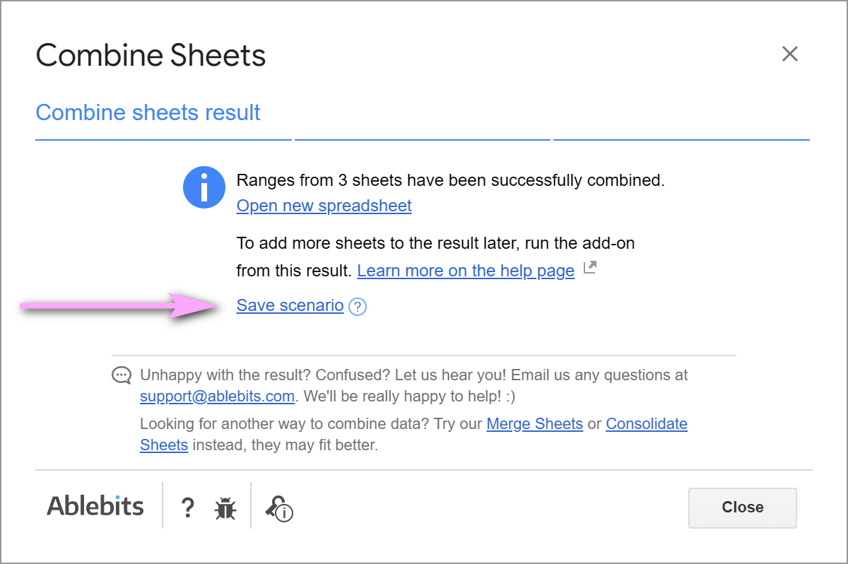
You will see your future scenario outline with the options you've just used. You can adjust a few of them to your convenience:
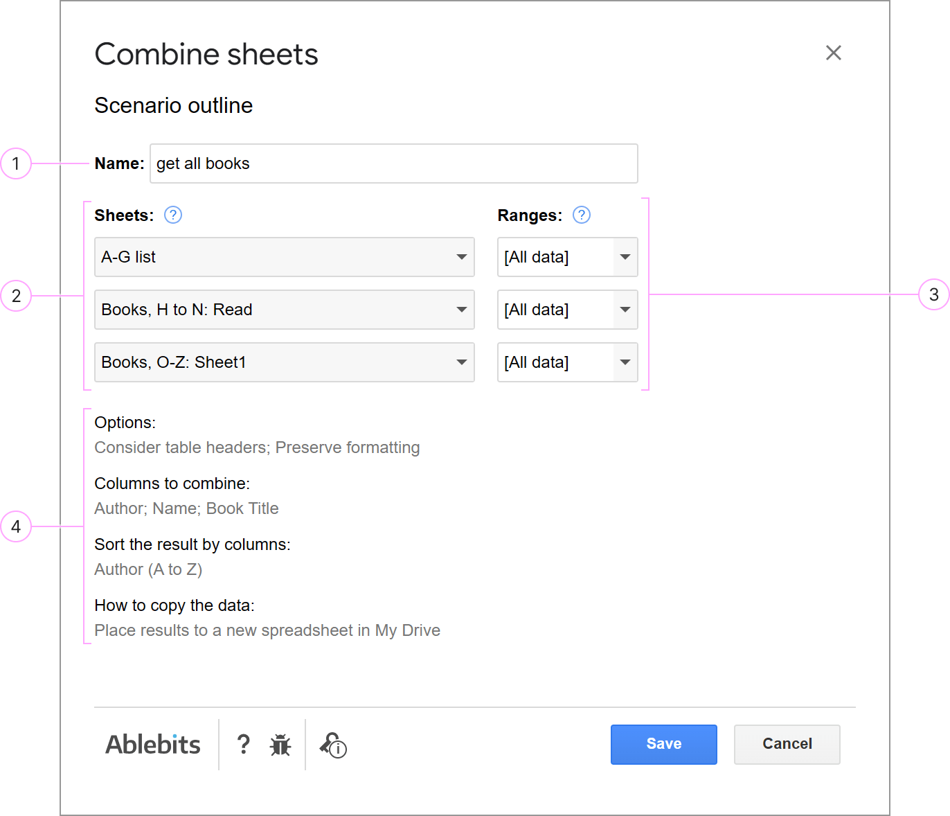
- Name your scenario in a way to understand what it does and find it among other scenarios quickly
- Select the sheets that will be combined each time you run the scenario:
- One of them can be [Selected sheet] — the sheet where you stand when running the scenario.
- Specify other sheets to always combine all data from them.
- Identify the exact ranges to combine the data from:
- Keep [All data] so the add-on automatically takes the entire used ranges for work.
- Go for [Selected range] to work with the cells you manually select before running the scenario.
- For the tool to handle the exact cells, simply enter the desired ranges of cells.
- Check if all other options you've just used are correct.
Note. You cannot change these options here. To modify them, please restart the add-on to pick the correct settings on steps 1-3.
Once everything's set, click Save and the scenario will be created.
Run your scenario
To start the scenario, go to Extensions > Combine Sheet > Scenarios, find the necessary name and click Start.
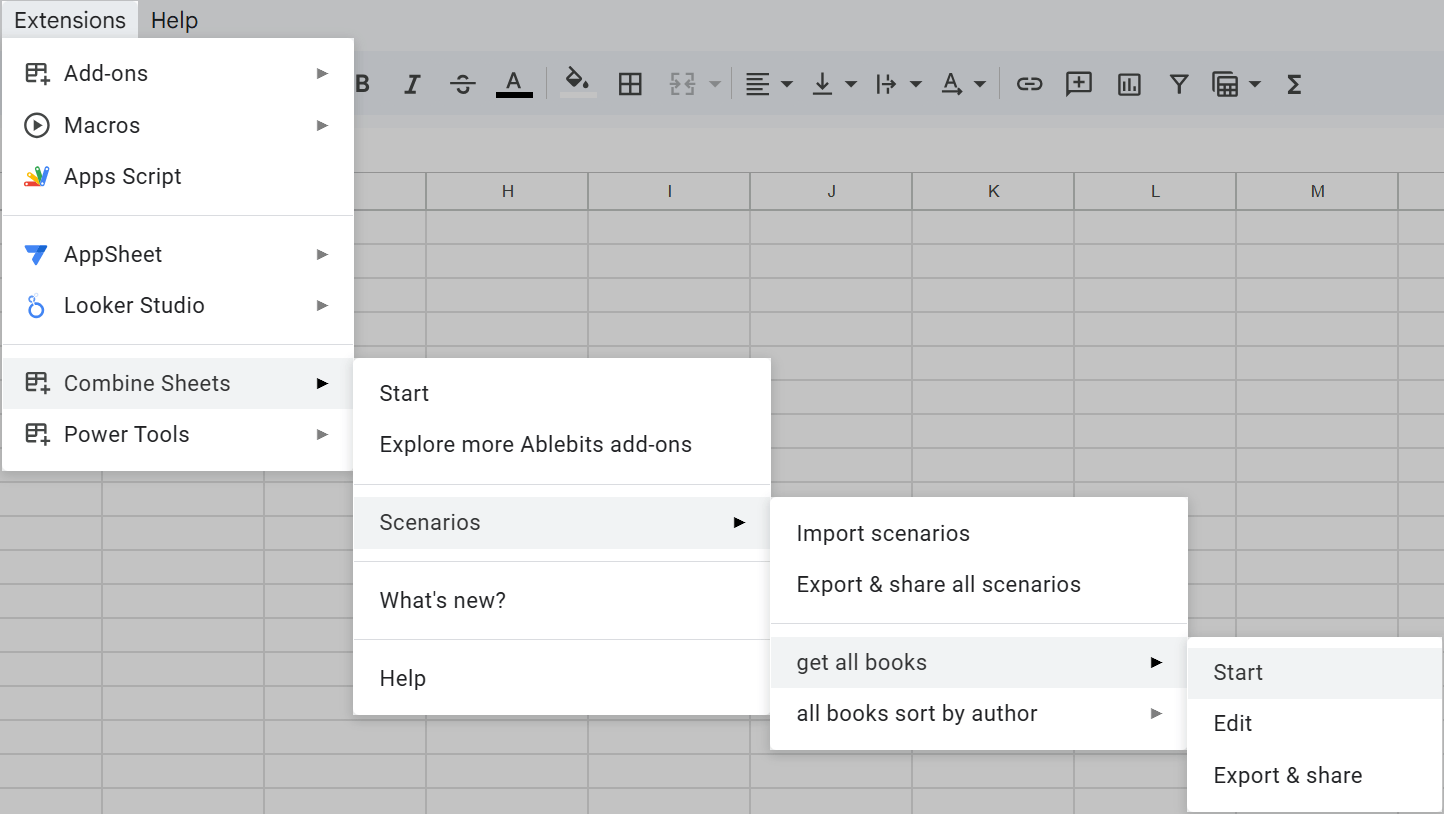
Note. If you don't see Scenarios in the menu, just click Extensions > Combine Sheets > Start to open the add-on itself once. This is necessary for new spreadsheets and those where the add-on hasn't been run yet. Your scenario (and all future ones) will then appear in the menu automatically.
This will run the tool and start processing your data right away per all the settings.
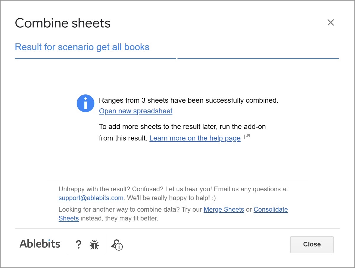
In the end, you will get the resulting message saying what scenario has been used, how many sheets have been combined and where to look for the result:
Edit or delete scenarios
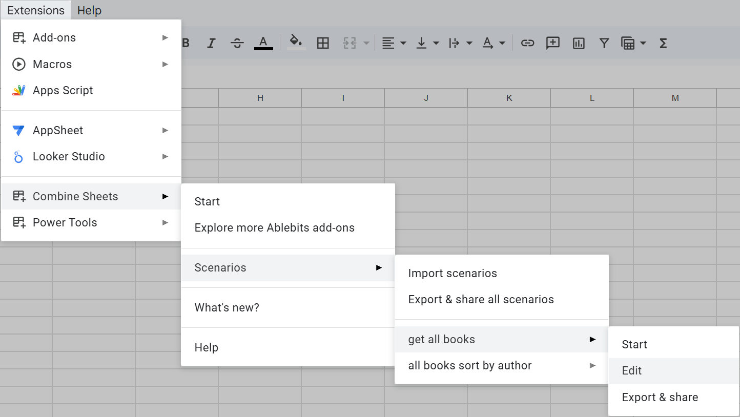
To edit your existing scenario, go to Extensions > Combine Sheet > Scenarios, pick the scenario and click Edit:
You will see the familiar scenario outline. The editable fields are the same: name, sheets, and data ranges:
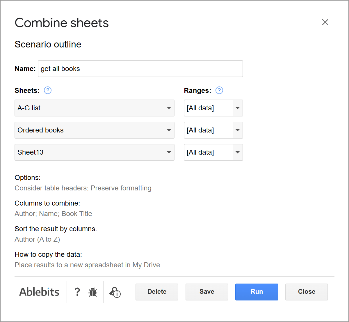
Press Delete to remove the scenario forever, Save to keep the changes, or Run to start it right away with the new settings.
Share scenarios
You can share all or only certain scenarios with your teammates or between your different Google accounts.
Share certain scenarios
To share only certain scenarios, go to Extensions > Combine Sheets > Scenarios > your scenario > Export & share:
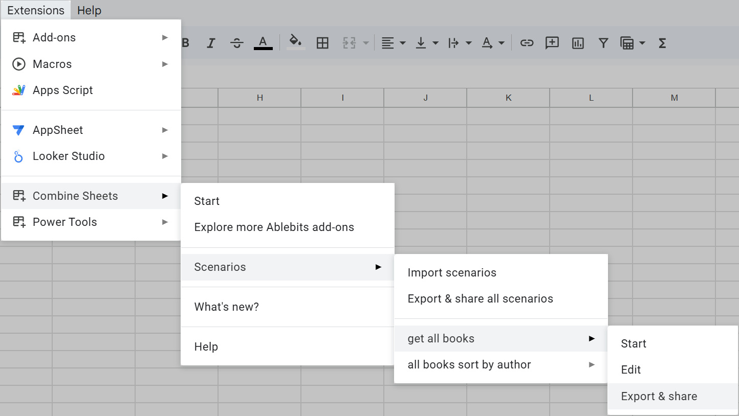
You will be prompted to save the scenario to your computer:
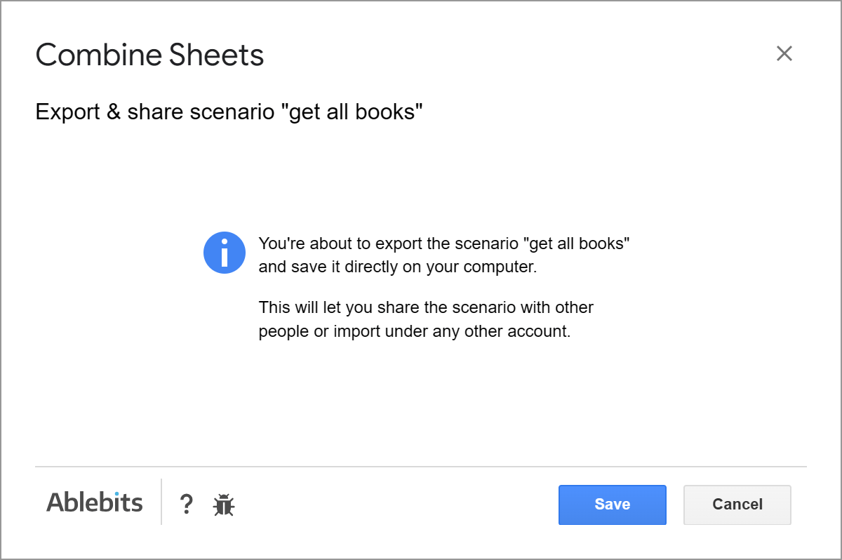
Click Save, and your browser will let you select a place where you'd like to save a file with a selected scenario. Once your browser downloads the file, you can close the add-on window.
Send this saved file to any Combine Sheets user so they could import it to their add-on and make use of this scenario.
Share all scenarios
To share all scenarios you've created, go to Extensions > Combine Sheets > Scenarios, and then right to Export & share all scenarios:

The add-on will let you know that you're about to save the file with all scenarios to your computer:
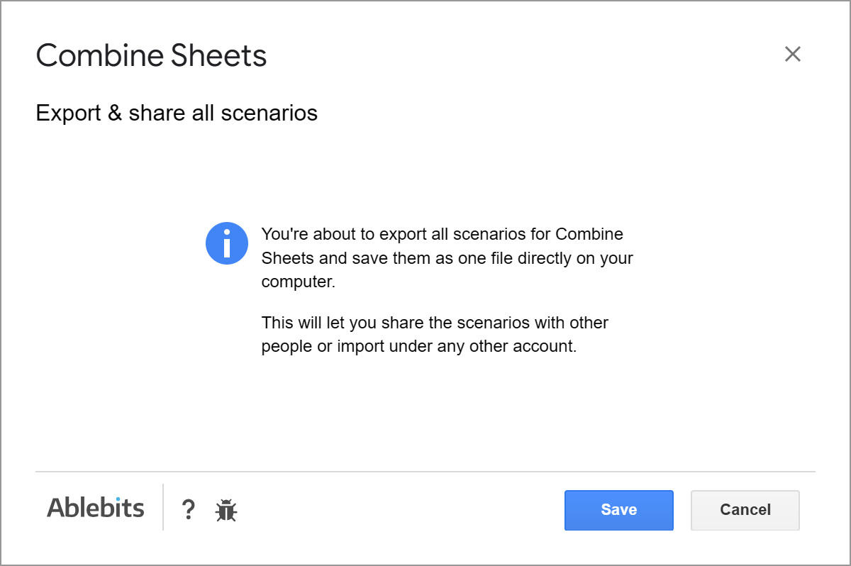
Click Save, and your browser will let you select a place where you'd like to save the file with scenarios. Once you download it, you can close the add-on window.
Send this saved file to any Combine Sheets user so they could import it to their add-on for future use.
Import scenarios
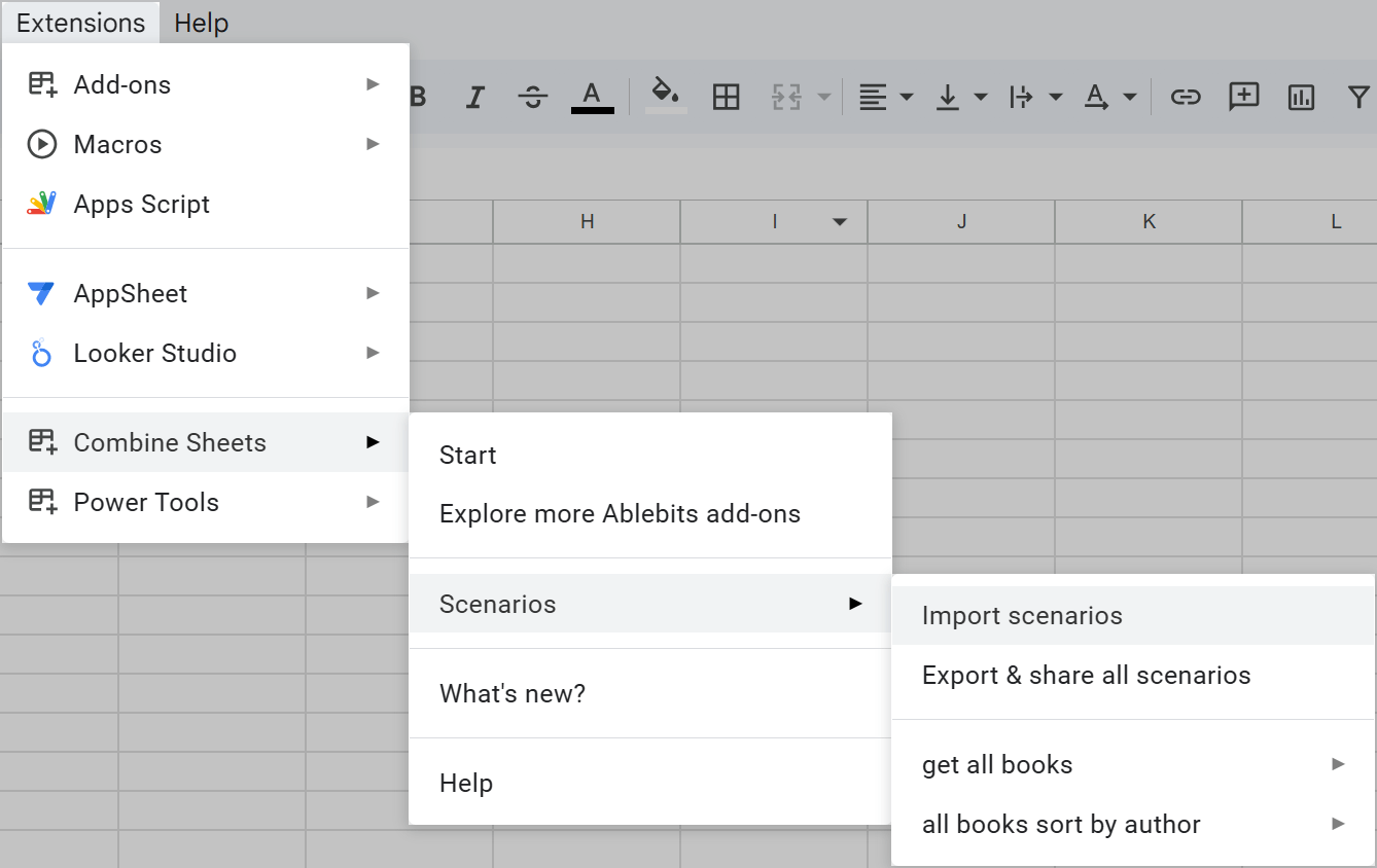
To import the scenarios someone has shared with you, go to Extensions > Combine Sheets > Scenarios > Import scenarios:
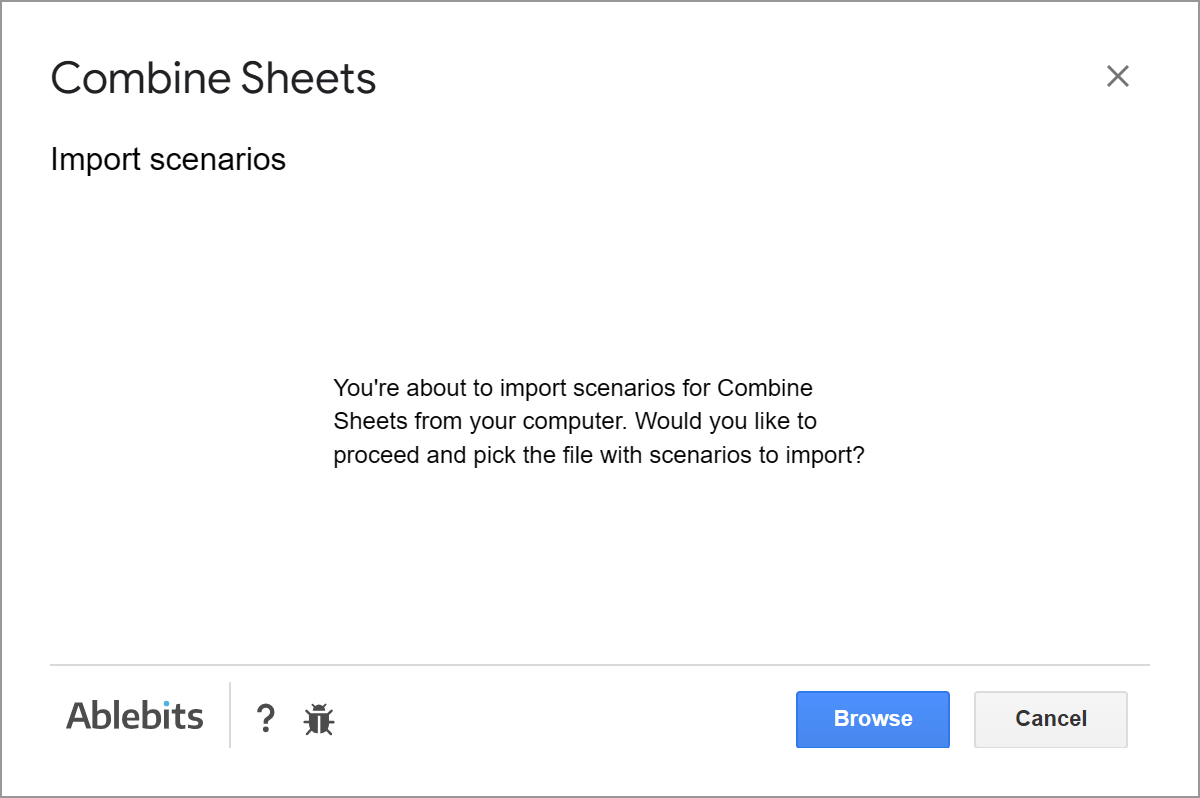
Combine Sheets will ask you to pick the file with scenarios from your computer using your browser File Manager. Click Browse to do that:
When you add the required file, the add-on will let you know how many scenarios from that file have been imported:
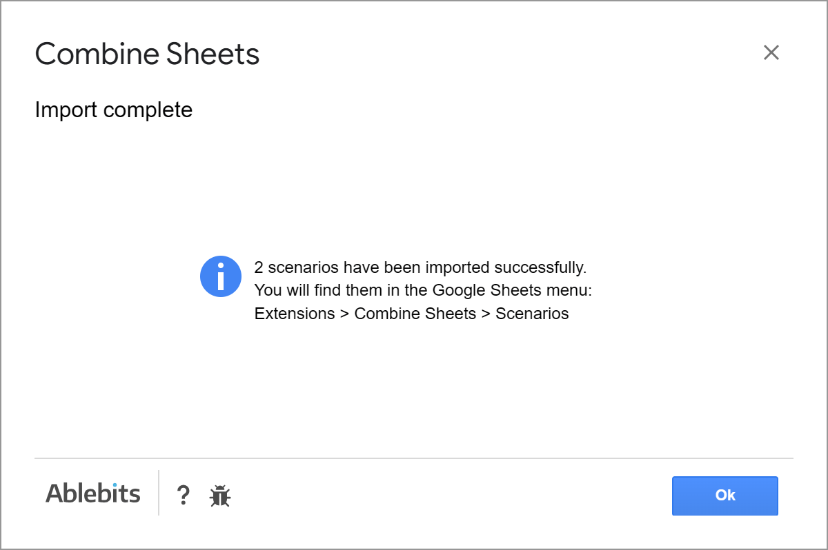
Tip. The add-on imports all scenarios from the files by default. But if you already have some of them or if something goes wrong, the add-on will inform you accordingly.
All imported scenarios will appear in your Combine Sheets > Scenarios menu:
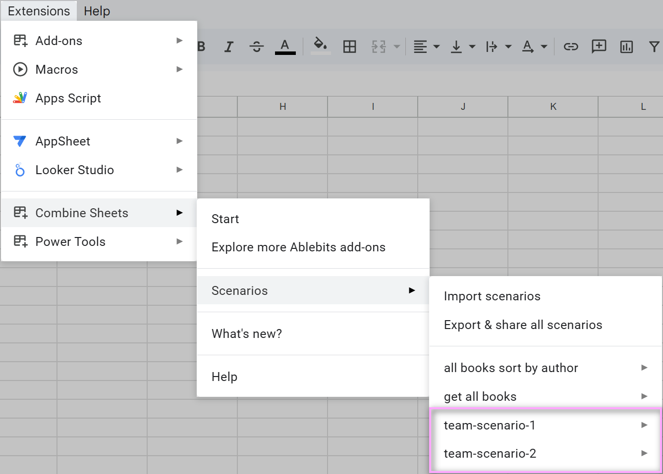
You can run them right away if you know what spreadsheets they're created for, or review and edit them beforehand.
Responses
Post a comment
Seen by everyone, do not publish license keys and sensitive personal info!