The tutorial shows how to use IF together with the AND function in Excel to check multiple conditions in one formula.
Some things in the world are finite. Others are infinite, and the IF function seems to be one of such things. On our blog, we already have a handful of Excel IF tutorials and still discover new uses every day. Today, we are going to look at how you can use IF together with the AND function to evaluate two or more conditions at the same time.
IF AND statement in Excel
In order to build the IF AND statement, you obviously need to combine the IF and AND functions in one formula. Here's how:
Translated into plain English, the formula reads as follows: IF condition 1 is true AND condition 2 is true, do one thing, otherwise do something else.
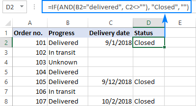
As an example, let's make a formula that checks if B2 is "delivered" and C2 is not empty, and depending on the results, does one of the following:
- If both conditions are TRUE, mark the order as "Closed".
- If either condition is FALSE or both are FALSE, then return an empty string ("").
=IF(AND(B2="delivered", C2<>""), "Closed", "")
The screenshot below shows the IF AND function in Excel:
If you'd like to return some value in case the logical test evaluates to FALSE, supply that value in the value_if_false argument. For example:
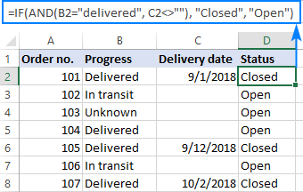
=IF(AND(B2="delivered", C2<>""), "Closed", "Open")
The modified formula outputs "Closed" if column B is "delivered" and C has any date in it (non-blank). In all other cases, it returns "Open":
Note. When using an IF AND formula in Excel to evaluate text conditions, please keep in mind that lowercase and uppercase are treated as the same character. If you are looking for a case-sensitive IF AND formula, wrap one or more arguments of AND into the EXACT function as it is done in the linked example.
Now that you know the syntax of the Excel IF AND statement, let me show you what kind of tasks it can solve.
Excel IF: greater than AND less than
In the previous example, we were testing two conditions in two different cells. But sometimes you may need to run two or more tests on the same cell. A typical example is checking if a cell value is between two numbers. The Excel IF AND function can easily do that too!
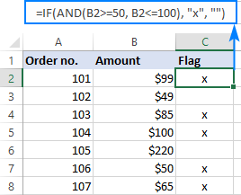
Let's say you have some sales numbers in column B and you are requested to flag the amounts greater than $50 but less than $100. To have it done, insert this formula in C2 and then copy it down the column:
=IF(AND(B2>50, B2<100), "x", "")

If you need to include the boundary values (50 and 100), use the less than or equal to operator (<=) and greater than or equal to (>=) operator:
=IF(AND(B2>=50, B2<=100), "x", "")
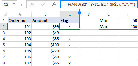
To process some other boundary values without changing the formula, enter the minimum and maximum numbers in two separate cells and refer to those cells in your formula. For the formula to work correctly in all the rows, be sure to use absolute references for the boundary cells ($F$1 and $F$2 in our case):
=IF(AND(B2>=$F$1, B2<=$F$2), "x", "")
By using a similar formula, you can check if a date falls within a specified range.
For example, let's flag dates between 10-Sep-2018 and 30-Sep-2018, inclusive. A small hurdle is that dates cannot be supplied to the logical tests directly. For Excel to understand the dates, they should be enclosed in the DATEVALUE function, like this:
=IF(AND(B2>=DATEVALUE("9/10/2018"), B2<=DATEVALUE("9/30/2018")), "x", "")
Or simply input the From and To dates in two cells ($F$1 and $F$2 in this example) and "pull" them from those cells by using the already familiar IF AND formula:
=IF(AND(B2>=$F$1, B2<=$F$2), "x", "")

For more information, please see Excel IF statement between two numbers or dates.
IF this AND that, then calculate something
Apart from returning predefined values, the Excel IF AND function can also perform different calculations depending on whether the specified conditions are TRUE or FALSE.
To demonstrate the approach, we will be calculating a bonus of 5% for "Closed" sales with the amount greater than or equal to $100.
Assuming the amount is in column B and the order status in column C, the formula goes as follows:
=IF(AND(B2>=100, C2="closed"), B2*10%, 0)

The above formula assigns zero to the rest of the orders (value_if_false = 0). If you are willing to give a small stimulating bonus, say 3%, to orders that do not meet the conditions, include the corresponding equation in the value_if_false argument:
=IF(AND(B2>=100, C2="closed"), B2*10%, B2*3%)

Multiple IF AND statements in Excel
As you may have noticed, we have evaluated only two criteria in all the above examples. But there is nothing that would prevent you from including three and more tests in your IF AND formulas as long as they comply with these general limitations of Excel:
- In Excel 2007 and higher, up to 255 arguments can be used in a formula, with a total formula length not exceeding 8,192 characters.
- In Excel 2003 and lower, no more than 30 arguments are allowed, with a total length not exceeding 1,024 characters.
As an example of multiple AND conditions, please consider these ones:
- Amount (B2) should be greater than or equal to $100
- Order status (C2) is "Closed"
- Delivery date (D2) is within the current month
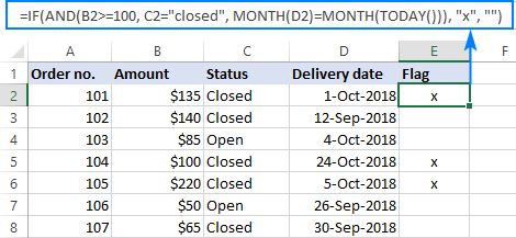
Now, we need an IF AND statement to identify the orders for which all 3 conditions are TRUE. And here it is:
=IF(AND(B2>=100, C2="Closed", MONTH(D2)=MONTH(TODAY())), "x", "")
Given that the 'current month' at the moment of writing was October, the formula delivers the below results:
Nested IF AND statements
When working with large worksheets, chances are that you may be required to check a few sets of different AND criteria at a time. For this, you take a classic Excel nested IF formula and extend its logical tests with AND statements, like this:
To get the general idea, please look at the following example.
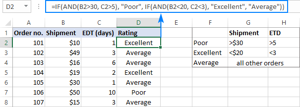
Supposing you want to rate your service based on the shipment cost and estimated time of delivery (ETD):
- Excellent: shipment cost under $20 and ETD under 3 days
- Poor: shipment cost over $30 and ETD over 5 days
- Average: anything in between
To get it done, you write two individual IF AND statements:
IF(AND(B2<20, C2<3), "Excellent", …)
IF(AND(B2>30, C2>5), "Poor", …)
…and nest one into the other:
=IF(AND(B2>30, C2>5), "Poor", IF(AND(B2<20, C2<3), "Excellent", "Average"))
The result will look similar to this:
More formula examples can be found in Excel nested IF AND statements.
Case-sensitive IF AND function in Excel
As mentioned in the beginning of this tutorial, Excel IF AND formulas do not distinguish between uppercase and lowercase characters because the AND function is case-insensitive by nature.
If you are working with case-sensitive data and want to evaluate AND conditions taking into account the text case, do each individual logical test inside the EXACT function and nest those functions into your AND statement:
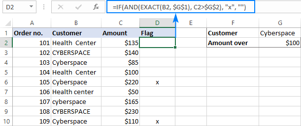
For this example, we are going to flag orders of a specific customer (e.g. the company named Cyberspace) with an amount exceeding a certain number, say $100.
As you can see in the below screenshot, some company names in column B look the same excerpt the characters case, and nevertheless they are different companies, so we have to check the names exactly. The amounts in column C are numbers, and we run a regular "greater than" test for them:
=IF(AND(EXACT(B2, "Cyberspace"), C2>100), "x", "")
To make the formula more flexible, you can input the target customer name and amount in two separate cells and refer to those cells. Just remember to lock the cell references with $ sign ($G$1 and $G$2 in our case) so they won't change when you copy the formula to other rows:
=IF(AND(EXACT(B2, $G$1), C2>$G$2), "x", "")
Now, you can type any name and amount in the referenced cells, and the formula will flag the corresponding orders in your table:
IF OR AND formula in Excel
In Excel IF formulas, you are not limited to using only one logical function. To check various combinations of multiple conditions, you are free to combine the IF, AND, OR and other functions to run the required logical tests. Here is an example of IF AND OR formula that tests a couple of OR conditions within AND. And now, I will show you how you can do two or more AND tests within the OR function.
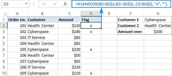
Supposing, you wish to mark the orders of two customers with an amount greater than a certain number, say $100.
In the Excel language, our conditions are expressed in this way:
OR(AND(Customer1, Amount>100), AND(Customer2, Amount>100)
Assuming the customer names are in column B, amounts in column C, the 2 target names are in G1 and G2, and the target amount is in G3, you use this formula to mark the corresponding orders with "x":
=IF(OR(AND(B2=$G$1, C2>$G$3), AND(B2=$G$2, C2>$G$3)), "x", "")
The same results can be achieved with a more compact syntax:
=IF(AND(OR(B2=$G$1,B2= $G$2), C2>$G$3), "x", "")
Not sure you totally understand the formula's logic? More information can be found in Excel IF with multiple AND/OR conditions.
That's how you use the IF and AND functions together in Excel. Thank you for reading and see you next week!
Practice workbook
IF AND Excel – formula examples (.xlsx file)
 by
by
458 comments
Dear Mam,
I have some problem in if functions.
if sales value is less than equal to 2 lakh then % incentive will be of 2.5% of net sales value.
if sales value is more than 2 lakh and less than equal to 5 lakh then % incentive will be 3% of sales value.
if Sales value is more than 5 lakh and less than equal to 10 lakh then % incentive will be 3.5% of sales value.
And if sales value is more than 10 lakh then % incentive will be 4% of sales value.
please suggest how to solve it.
With regards,
I need help with a multiple IF /IF AND formula because I am totally lost here.
I have 5 colons I need to take in my formula, with a total of 4 conditions and I need to calculate the following:
IF(AND(D1460, G14=0) then D14*$L$10,
IF(D14+G14<=59, then $M$9,
IF(AND(G14=<60, P14=J), then D14*$L$10+$M$9,
and in all other cases it should be D14+G14
How do I get them all in one field and make excel calculate the result with all those parameters? Is it possible at all? I tried with:
IF((AND(D1460, G14=0), D14*$L$10, IF(D14+G14<=59, $M$9, IF((AND(G14=<60, P14=J), D14*$L$10+$M$9, D14+G14)))) But the formula is obviously wrong :-(
Since I am a linguist and the last time I had maths was in 1983, you can understand my confusion... Many thanks!
Hi Maria,
It looks like you might have some overlaps for solutions is why it might not be working.
Could you list the range of values the cells could have?
I need one equation.
One cell contain one value suppose 100 i need in next in following conditions.
25 percentage of 100 plus 4 percentage of coming answer of 25 percentage.
=(A1*25%)+(A1*25%*4%)
You can also have the percentages in their own columns that way if you want to adjust, you can just change the values in the reference columns.
=(A1*$B$1)+(A1*$B$1*$C$1)
ExtMatlGrp Frm Lot to lot Scrap %
100-34 0 2 250
100-34 2.001 5 65
100-34 5.001 10 25
100-34 10.001 50 9.75
100-34 50.001 100 9.75
100-34 100.001 200 8.75
100-34 200.001 999999 6.25
100-48 200.001 999999 5.75
100-48 100.001 200 6.75
100-48 50.001 100 9
100-48 10.001 50 13.5
100-48 5.001 10 25
100-48 2.001 5 65
100-48 0 2 250
101-120 0 2 250
101-120 2.001 5 65
101-120 5.001 10 25
101-120 10.001 50 14.5
101-120 50.001 100 12
101-120 100.001 200 9
101-120 200.001 999999 8.25
102-104 200.001 999999 11.25
102-104 100.001 200 13.75
102-104 50.001 100 14
dear sir my coloum is fix it is not vary but my 2nd coloun and 3rd coloum lot size is varying example 0-2 is 250 suppose if i put excel arrangemnt like 1 then automatically comes out 250%
Range, greater than and less than in the formula are showing as O. So, I am adding the statements to clarify.
IF(AND((G3+2*$I$1) less than range C3 to C6, V3 greater than 0, IF(V3="NP","NF1",1))
IF(AND((G3+2*$I$1)0,0,IF(V3="NP", "NF1",1))
The below formula is trying to fill a range instead of just one cell. What is the error?
=IF(AND((G3+2*$I$1)0,0,IF(V3="NP","NF1,1))
I have to get output value based on the below scenario
Target qty(T) Achived qty(A) % Achived (A.P) Output value (O.V)
200 200 100%
Conditions : If achieved % is >90% and <100% then outvalue should be such that for every decrement of achieved % 2% should be deducted (eg: if % Ach is 98% then Output value should be 96%, if Ach % is 90% and <100% 2% deduction and from <90%, 1.5% deduction.(eg: If achi. 85% then output value should be 72.5% (upto 90%,2% reduction, 100%, then for every increment 2% increase.(Eg: Ach% is 102% the output value should be 104%)
I have tried building formula using if & netsed if& and formula but I didn't got the right formula. please help to build the formula in excel to get output in the mentioned conditions
I have to get an output based on the below scenario.
Target Achieved %Ach
i have some data where i found some value i have return header with concatenate the header value.
Mismatch - Recipient GSTIN Mismatch - GSTIN of the Supplier Mismatch - Invoice/Debit Note/ Credit Note (No) Mismatch - Invoice/Debit Note/ Credit Note (Date) Mismatch - Original Invoice No Mismatch - Original Invoice Date Mismatch - POS Mismatch - Supply attract reverse charge Mismatch - Total GST Rate Mismatch - Taxable Value Mismatch - IGST (Amt) Mismatch - CGST (Amt) Mismatch - SGST/UTGST (Amt) Mismatch - Cess(Amount)
No No No No No Yes Yes No No No Yes Yes Yes No
No No No yes No Yes Yes No No No Yes Yes Yes No
i have to use three conditions in a cell. for example if A1500, result will be TRUE , if A1<-500, result will be NEGATIVE.
NOTE: the third condition is negative value (- 500)
can you please help me to do this
i have to use three conditions in a cell. for example if A1500, result will be false, if A1<-500, result will be negative.
NOTE: the third condition is negative value (- 500)
can you please help me to do this
Huge help, thank you very much!
I have a formula issue, below need help;
If A3 shows “any value”, show D3 as “In Progress”
If A3 and E3 shows “any value”, show D3 as “Completed”
If A3 and I3 shows “any value”, show D3 as “Pending Approval” < Particular this one having trouble with as the rest work in below formula. I’m close the issue is that this shows “In Progress”
If A3 and E3 shows “blank” show D3 as “Blank”.
This is the formula in its current value, any chance you could take a look and see if there is something wrong?
=IF($A3"",IF($E3"","Completed","In Progress"),IF($A3"",IF($E3="",IF(AND($I3"","Pending Approval","In Progress"),"Completed")),""))
=IF(AND(A3"",E3="",I3=""),"IN PROGRESS",IF(AND(A3"",E3"",I3=""),"COMPLETED",IF(AND(A3"",E3="",I3""),"PENDING APPROVAL",IF(AND(A3="",E3=""),""))))
I am trying to include a formula in excel where if "EUROS" is entered in one cell the next cell will populate the € symbol but will also include the value that I enter.
What formula would I need for this?
Hi Sally,
Please try the formula below.
=IF(A1="EUROS","€"&B1)
I want a formula that will write 1/10/2019 - 2/10/2019 in a cell, if a particular condition lets say a1:a30 is WK1
This should mean that 1st is WKI, and 2nd is also WK1
Hi,
I have a list of 12 different countries in one column and 38 different statements in another column. I'm stuck trying to get the following results basded on all possible combinations (456!) sourcing from different spreadsheets.
IF Argentina + Football then Column X
IF Brazil + Tennis then Column Y
If Argentina + Tennis then Column Z....and so on.
I've been using this formula (=+IF(AND(EXACT(A3;TEST!A2);EXACT(C3;TEST!C2);TEST!E2<30%);TEST!D2;TEST!E2), which is close but every time I change the order of the rows, the results change so, actually, my formula is not working because, for instance, the result of Argentina + Football would appear as Z instead of X.
May you help me, please?
I have a spreadsheet with list of schools and states. Column G lists the state abbreviation and I have 13 analysts. I would like a blanks column B to pre-fill with an assigned analyst name based on their assigned states. For example I tried =IF(G6="NC", "Jay", IF(G6="MT", "Jay", IF(G6="FL", "Rami", IF(G6="VT", "Rami", IF(G6="TX", "Joe"))))...... but I get a warning there are two many arguments.
Any suggestion?
Thanks,
J
Hi Jay,
I would try the Excel IFS function instead:
=IFS(OR(G2="MT",G2="NC"),"Jay",G2="TX","Joe",OR(G2="FL",G2="VT"),"Rami")
I have this Data how to solve?
Grade>=17 And Sex =F And Location it is Bhandup, Mulund, 10% on Basic, Grade>19, 20% on basic , otherwise 8%
Hi Ravina,
Condition 1 and Condition 2 seem to be overlapping in your task. However, the following formula may serve as a starting point and can easily be modified if you decide to alter the conditions:
=IFS(B2>19,20,AND(B2>=17,C2="F",D2="Bhandup, Mulund"),10,TRUE,8)
PS If you wonder why there is ‘TRUE’ before 8 there, press ‘F1’ to search for the Excel IFS function, and you will find the answer. That’s where I learnt it myself.
Hi Everyone! I'm building an estimating spread sheet and I'm having "#Value!" issues with what should be a very simple process. In my case Columns A & B contain a drop down menu. In column A there is only one appropriate choice, let's say "Floor". In column 2 there can be up to three appropriate choices, "Bathroom", "Ensuite" & "PWD" from which, obviously, only one is chosen. In simple English the process is this:
IF cell A1 = "Floor" & cell B1 = "Ensuite", multiply cells F1*G1*O1, otherwise return "" blank.
Of course cell B1 might read "Bathroom, "Ensuite" or "PWD" so this needs to be included in the formula. My problem appears to be incorporating these 3 variables for that cell and I can't find a way around it. Any help that you can give would be greatly appreciated!
Many thanks,
Dick
=IF(AND(A1="FLOOR",OR(B1="BATHROOM",B1="ENSUITE",B1="PWD")),F1*G1*O1,"")
That one should work
=IF( orand(A2>89 , A2<199) , "a"; IF( A2=1, "2"; IF( A2=200, "ok" ; " no " )))
I have this data:
KEY A B C D E F G H I J
3323 6 66 86 64 20 89 68 42 16 31
3324 5 17 46 36 9 40 72 62 81 68
3325 62 8 44 18 80 52 6 55 3 66
3484 37 29 31 67 57 55 2 50 12 28
3485 32 33 49 80 29 77 30 18 68 78
3486 59 11 55 41 62 71 72 70 1 68
I WANT TO USE THE IF AND FORMULA TO CHECK IF I GET 2 NUMBER THAT ARE THE SAME THEN
I WANT TO THE KEY AND THAT NUMBERS. FOR EXAMPLE KEY 3323 HAS 6, 66 SO IS KEY 3325 SO THERE IS A MATCH. THE OUTPUT WILL BE 3323 6 66 86 64 20 89 68 42 16 31
3525 62 8 44 18 80 52 6 55 3 66
ANOTHER MATCH IS 3324 5 17 46 36 9 40 72 62 81 68
3486 59 11 55 41 62 71 72 70 1 68
WE HAVE 6-66 AS A MATCH IN 3323 AND 3525 AND ANOTHER MATCH IN 72-68 IN 3324 AND 3486
I ALSO WANT TO USE THE VLOOKUP OR ANY OTHER FORMULA A THAT WILL DO THE SEARCH AND A MATCH. I AM A BEGINNER, AND STILL LEARNING, ANY HELP OUT THERE?
Hi
I'm trying to achieve what I believe the be a IF AND OR formula please. This is what I have so far:
=IF((AND(B3="linux/Unix",D5="Run the following network scan:")),"nmap -A ","1..255 | % {echo ''192.168.X.$_''; ping -n 1 -w 100 192.168.X.$_} | Select-String ttl")
B3 is a drop box so if "Linux/Unix" is not selected, then Windows is the only other option which displays the second outcome.
However, I want to add an extra piece =if(D5="Next Question", " ", " "). Basically I want a black cell left if D5="Next Question" regardless of what B3 equals please.
I have tried adding this to the end with extra brackets, but this does not work and I'm not sure where else to nest it please?
=IF(D5="NEXT QUESTION","",IF(AND(B3="linux/Unix",D5="Run the following network scan:"),"nmap -A ","1..255 | % {echo ''192.168.X.$_''; ping -n 1 -w 100 192.168.X.$_} | Select-String ttl"))
That should work
Pls help me get a formulae for calculating the rate(%) for a particular deposit given the amount and period using the below tables:
Fixed deposit of 10 to 50M. Rate;
30 to 90 days - 6.50%
91 to 180 days - 7.00%
181 to 365 days - 7.25%
Fixed deposit of >50M. Rate;
30 to 90 days - 7.00%
91 to 180 days - 7.25%
181 to 365 days - 7.50%
what if im looking for an IF THEN in a range,
example
IF in this range "x" is found THEN do this
Can you please give a correct formula for the below
IF SHEET2 COLUMN B VALUE = SHEET1 COLUMN B VALUE AND (ITS) SHEET1 COLUMN D VALUE= POSTED OR HOLD THEN COLUMN C VALUE ADDED TO COLUMN H
IF SHEET2 COLUMN B VALUE = SHEET1 COLUMN B VALUE AND (ITS) SHEET1 COLUMN D VALUE= DELIVERED OR TRANSIT THEN COLUMN C VALUE ADDED TO I
I have 2 scenario's which have 2 diff IF statements. I need this to be in the same cell and cannot get it to work. Any suggestions.
IF(AND(J4="MOLCO",Y4="SHORE",W4>S4),"-",S4-W4)
IF(AND(J4="MOLOO",Y4="SHORE",W4>U4),"-",U4-W4)
In both statements if all the AND(.....) are true then it only needs to return "-".
Thanks
Michael
=IF(AND(J4="MOLCO",Y4="SHORE",W4>S4),"-",IF(OR(J4"MOLCO",Y4"SHORE",W4U4),"-",IF(AND(J4"MOLOO",Y4"SHORE",W4<U4),U4-W4,""))))
It's a little messy but, this should work.
IF(OR(J4"MOLCO",Y4"SHORE",W4<U4)
The formula is missing "" back to back. Not sure why it won't show up.
Less than "" back-to-back.
so, for my homework im supposed to do this:
In cell B10, enter a formula using the IF and AND functions to indicate whether the revenue goal has been met that month:
a. Enter the logical test using the AND function to determine if the Fundraisers amount in cell B7 equals 0 and the Total in cell B8 is greater than 20000.
b. If the logical test is true, display Yes (using “Yes” for the value_if_true argument).
c. If the logical test is false, insert a nested IF function.
d. Enter the logical test of the nested IF function using the AND function to determine if the Fundraisers amount in cell B7 is greater than 0 and the Total in cell B8 is greater than 200000.
e. If the logical test for the nested IF function is true, display Yes (using “Yes” for the value_if_true argument).
f. If the logical test is false, display No (using “No” for the value_if_false argument).
but i cant get it to work. i tried making this formula:
=IF(AND(B7=0,B8>20000),Yes,IF(AND(B7>0,B8>200000),Yes,No))
but it only gives a result of #NAME?
you can try this
=IF(AND(A7=0,B7>20000),"Yes",IF(AND(A7>0,B7>200000),"No"))
=IF(AND(L11>=30, L11<100), "OBESE", IF(AND(L11=25), "OVERWEIGHT", IF(AND(L11>25, L11>=18.5), "NORMAL WEIGHT", IF(AND(L110), "UNDERWEIGHT")))))
Hi Patrick,
If I get it right, you mean the following:
1) an ‘OBESE’ note is required if the value in L11 is equal to or more than 30 but less than 100;
2) an ‘OVERWEIGHT’ note is required if the value in L11 is equal to 25;
3) a ‘NORMAL WEIGHT’ note is required if the value in L11 is equal to or more than 18.5 but less than 25;
4) an ‘UNDERWEIGHT’ note is required if the value in L11 is equal to 0.
If so, I would rewrite your formula applying the IFS function:
=IFS(L11=0, "UNDERWEIGHT", AND(L11>=18.5, L11<25), "NORMAL WEIGHT", L11=25, "OVERWEIGHT", AND(L11>=30, L11<100), "OBESE")
Please note that the above formula will bring ‘#N/A’ every time you try to make it process values like 15, 27, or 102 since they are not covered by your conditions.
Can someone tell me what's wrong with this formula, I can't seem to get it to work. Thanks!
=IF(AND(L11>0, L11=18.5, L11=25, L11=30, L11<100, "Obese"))))))))
That's not the formula I wrote, hang on...
Im looking for a formula that works for this:
=IF(AND(B6="yes",OR(C6>7am,C6<3pm)),"yes","no")
I have tried a combination of if, and and or together and =time(7,0.0) and it only returns the first logical test. Im losing sleep over it!
If cell b6 = yes
And
Cell c6 is less than 7am or greater than 3pm
Return yes value.
IF A is greater than 1000 and lesser than 2000 then figure should display of "A" CAN YOU SHARE THE FORMULA FOR THE SAME
I am trying the following formula and i get an error, can you help?
=IF(LEFT(D28,2)="SS",MID(D28,5,1)&"X",LEFT(D28,2),IF(OR(LEFT(D28,2)="OJ",AND(F28="1113"),"OJ1")))
my input looks like this, in K i would like to see OJ1, when D is OJ and F is 1113. the first part of the nested commands works fine.
D F K
OJDS01 1113 OJ1
SSDSC1 CX
i want formula for the followings:
1.ifSalary Rs.7000 =Lessthan than salary <7000*8.33%
2.7001 to 21000 salary (533.33/31days * no of worked days.
3.above 21000 =(833.33/31days* no.of.worked days.
kindly help me.
I've created a conduit fill schedule where if you select a conduit type the conduit type and the conduit size you get the conduit area number associated with that specific conduit type and trade size. In cell G, you can choose the conduit type via a drop down list. In cell F you enter the conduit size. In cell K depending on the selected conduit type (cell G) and the conduit size (cell F) you get the conduit area number for (cell G) & (cell F). My conduit types are PVC 40,PVC 80,RMT,EMT, & LFMC. When I combine IF with Vlookup in cell K the conduit area number is for PVC 40 only, the cell doesn't recognize the other conduit types.
How do I solve this?
Thank You for your expertise.
Hi,
I am trying to use match formula to give me the row where a formula applies too 10 cells. Eg if the cell number stays bellow 4.5 for 10 cells then give me the row this happens in. But how would i write 10 cells. As so far i have match(value, array, match type) but i need to put in only if applies to the following 10 cells.
Any thoughts?
the moving ribbon on the bottom of the blog page is crap, cant read because of that stupid thing
I have a list of customers each with a unique ID number
I can have the same customer multiple times on a report
Each Customer has a status of Ordered or Ordering
Using the customer number I need to know which customer number has both "Ordered" & "Ordering" in its status field.
The Result should be a Yes or No.
Hi Rich,
Let’s say your customers’ ID numbers are in Column A and the information on their status, which is either ‘Ordered’ or ‘Ordering’, is in Column C. I would suggest applying Ablebits’ ‘Merge Duplicates Wizard’ first to keep only unique ID numbers in Column A and a summed up record saying ‘Ordered;Ordering’ or ‘Ordering;Ordered’ in Column C. Don’t omit the ‘Backup this worksheet’ option so as not to lose your original table. Then I would write the following formula in Cell, say, H21:
=IF(AND(H20=INDEX(A:A,MATCH(H20,A:A,0)),OR(INDEX(C:C,MATCH(H20,A:A,0))="Ordered;Ordering",INDEX(C:C,MATCH(H20,A:A,0))="Ordering;Ordered")),"Yes","No")
That formula reacts to changing an ID number in Cell H20 and brings either “Yes” or “No”, depending on the situation. If you try to type in the ID number which Column A does not contain, the formula will bring ‘#N/A’.
or to go simpler
COL A COL B COL C COL D
ROW 1 Customer ID Ordering Ordered Both
ROW 2 1111 yes yes yes
IN D2 put the following formula: =IF(AND(B2="yes",C2="yes"),"yes","no")
then just simply copy and paste it down the Column D
:)
I have the following scenario which I can't seem to get the IF(OR(AND to work. I have an employee database that lists the name, title and location. I am using the above formula to determine security groups and distribution groups. I have come across a scenario where I have multiple titles with multiple possible locations. I currently have the following formula, which comes back with findings but they are inaccurate. =IF(OR(B3="OCT TECH - OCT Technician",B3="TECH - Ophthalmic Technician",B3="SCRIBE - Ophthalmic Scribe",B3="CLMANG - Clinic Manager",B3="OPTAST - Ophthalmic Assistant",B3="VFTECH - Visual Field Technician",B3="SPTEST - Special Testing Technician",B3="SXCORD - Surgical Coordinator",B3="DOCTOR - Medical Doctor",B3="OPTOM - Optometrist")*AND(C2="HAGER - Hagerstown",C2="Fred - Frederick",C2="HANCO - Hancock",C2="MARTI - Martinsburg"),"YES","NO") Any ideas? Thank you
currently have =IF(AND(F3>=D5,F3<=E5),”X”,””). This is checking to see if F3 is between two dates and if so to put an X in the cell otherwise leave blank. I want to add to that formula IF F3 is 1 day past E2 (which is a end date of project), or is 2 days past E2, then put a W. How might I accomplish this?
what is nested if function
I'm trying to use the IF statement to produce a value for three different cells that are equal to use that equal number. if they are not equal use the lowest value of the three.
ex.
IF('TRAINING TRACKER'!E3='TRAINING TRACKER'!M3='TRAINING TRACKER'!W3,"count#","count lowest#")
What do I need to use to produce a numeric value for each instance?
Hi there!! This is really long, but I am looking for a formula that would handle all of this
If column E = Eagle and column D = Select 6 and column P = 0-75 then column Q = 1.5%
If column E = Eagle and column D = Select 6 and column P = 76-80 then column Q = 1.1%
If column E = Eagle and column D = Select 6 and column P = 81-85 then column Q = .75%
If column E = Eagle and column D = Platinum 5 or Platinum 7 and column P = 0-75 then column Q = .75%
If column E = Eagle and column D = Platinum 5 or Platinum 7 and column P = 76-80 then column Q = .50%
If column E = Eagle and column D = Platinum 5 or Platinum 7 and column P = 81-85 then column Q = .38%
If column E = Symetra and column D = Edge GPS 5 or Edge GPS 7 then column Q = 1%
If column E = Symetra and column D = Advantage Income, Custom 5, Custom 7, Select 5 or Select 7 then column Q = .5%
This is very nice lesion. thank for teaching us. I have a question as below.
Below is the formulas I use as an example, but I got one error with the latest formulas, please assist to let me know what happened on this or because using wrong.
=IF(AND(B4<=25000,C4<=45),"Med N1",IF(AND(B4=46),"Med N3",IF(AND(B4=46),"Med N4",IF(AND(B4>=50001,C4=50001,C4>=46),"Med N5",IF(AND(B4>=100000,C4=100001, C4>=46),"Med N6","")))))))
I would like to ask why this below condition not apply?
IF(AND(B4>=100001, C4>=46),"Med N6","")
Help, how can I do a formula for the following condition: I have cells B3-D6 which will have an "x" (columns) as reply to four questions (rows). I want the fifth row to automatically add the" x" to be the total of the "X" only if it equals to four or three x's in a column. If a column equals 2 or less, nothing should be done. I would truly appreciate any assistance. Thanks.
i need a help in excel which can identify 2 different set of line example 1 Tin - Arrow gold - 5 K Seeds - 7400 Rs 1 Pkt - Broccoli Saki - pkt - 510 " this is in single cell but i want to highlight the same pls advice
Dear Sir,
I would like count no of cells having specific text for a specific employee with drop down list excluding blank cells.Here we are giving work sheet with data for your reference.
S.NO Employee Name FRI SAT SUN MON TUE WED THU FRI SAT SUN MON TUE WED THU FRI SAT SUN MON TUE WED THU FRI SAT SUN MON TUE WED THU FRI SAT
26 27 28 29 30 1 2 3 4 5 6 7 8 9 10 11 12 13 14 15 16 17 18 19 20 21 22 23 24 25
1 M.SANKAR G G G G G G G G G G G G A G G G G G A G G G G G
FABRICATOR B½ B G½
2 K.MURALI G G G G G G G G G G G G G G G G G G G G G
WELDER B½
3 M.VENKATRAMAIH G G G G G G G G G G G G G G G G A G G G G G G
WELDER B½ G½
4 M.RAMACHANDRA G G G G G G G G G G G G G G G G G A G G G G
KALASI B½ G½ B½
Thanks & regards,
Ramesh
Hi, good day
How can I horizontally lookup rate from a table (using index match) with 2 conditions.
This is my data set
Name 30-Nov-17 03-Jan-18 01-May-18 31-Oct-18
Andy 10% 8% 10% 8%
Sarah 10% 8% 10% 8%
James 10% 8% 10% 8%
John 10% 8% 10% 8%
I want to pick out the rates from the table based on Name and Effective Date. Eg., James / 15-Jan-18 would return "8%".
Many thanks
Thanks, svetlana.
for sharing.
Thanks for your great work you do by helping others..
I have a unique problem seeking formula for use in Office 2010.
Problem: Looking for a formula to :- Find matches in any two cells in the same row where.. For example column A has exactly five or 8 digit numbers and column B has only a single digit with result in column c stating match/no match
Say.. i have two columns in Excel each having numbers.In the first column A i have 5 or 8 number digits exactly. in B i have a single digit. what i need to do is find if the number present in column B, is matching in column A with result in column c stating match/no match i have enjoyed your formula given "Example 2. Find matches in any two cells in the same row
If you are looking for a way to compare columns for any two or more cells with the same values within the same row, use an IF formula with an OR statement: =IF(OR(A2=B2, B2=C2, A2=C2), "Match", "") " ...... But not helping with my problem Please reply. thanks
How to solve this?