Today we'll look at how to use VLOOKUP in Excel with many detailed step-by-step examples. You'll learn how to Vlookup from another sheet and different workbook, search with wildcards, and a lot more.
This article begins a series covering VLOOKUP, one of the most useful Excel functions and at the same time one of the most intricate and least understood. We will try to explain the basics in a very plain language to make the learning curve for an inexperienced user as easy as possible. We will also provide formula examples that cover the most typical usages of VLOOKUP in Excel, and try to make them both informative and fun.
Excel VLOOKUP function
What is VLOOKUP? To begin with, it is an Excel function :) What does it do? It searches for the value you specify and returns a matching value from another column. More technically, the VLOOKUP function looks up a value in the first column of a given range and returns a value in the same row from another column.
In its common usage, Excel VLOOKUP searches through your data set based on the unique identifier and brings you a piece of information associated with that unique identifier.
The letter "V" stands for "vertical" and is used to differentiate VLOOKUP from the HLOOKUP function that looks up a value in a row rather than column (H stands for "horizontal").
The function is available in all versions of Excel 365 through Excel 2007.
Tip. In Excel 365 and Excel 2021, you can use the XLOOKUP function, which is a more flexible and powerful successor of VLOOKUP.
VLOOKUP syntax
The syntax for the VLOOKUP function is as follows:
Where:
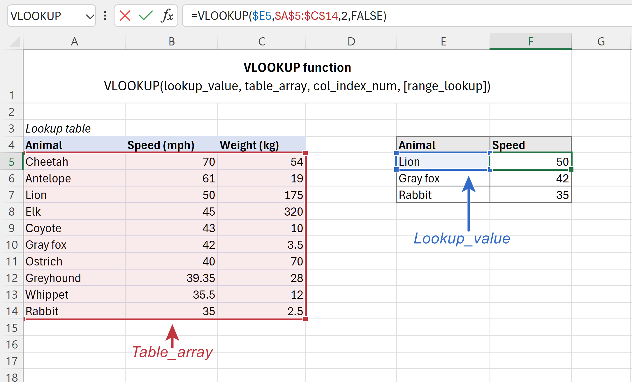
- Lookup_value (required) - is the value to search for.
This can be a value (number, date or text), cell reference (reference to a cell containing a lookup value), or the value returned by some other function. Unlike numbers and cell references, text values should always be in enclosed in "double quotes". - Table_array (required) - is the range of cells where to search for the lookup value and from which to retrieve a match. The VLOOKUP function always searches in the first column of the table array, which may contain various text values, numbers, dates, and logical values.
- Col_index_num (required) - is the number of the column from which to return a value. The counting starts from the leftmost column in the table array, which is 1.
- Range_lookup (optional) - determines whether to search for approximate or exact match:
- TRUE or omitted (default) - approximate match. If an exact match is not found, the formula searches for the largest value that is smaller than the lookup value. Requires sorting the lookup column in ascending order.
- FALSE - exact match. The formula searches for a value exactly equal to the lookup value. If an exact match is not found, a #N/A value is returned.
Basic VLOOKUP formula
Here is an example of the Excel VLOOKUP formula in its simplest form. Please have a look at the below formula and try to "translate" it into English:
=VLOOKUP("lion", A2:B11, 2, FALSE)
- The 1st argument (lookup_value) clearly indicates that the formula looks up the word "lion".
- The 2nd argument (table_array) is A2:B11. Keeping in mind that the search is performed in the left-most column, you can read the above formula a little further: search for "lion" in the range A2:A11. So far, so good, right?
- The 3rd argument col_index_num is 2. Meaning, we want to return a matching value from column B, which is second in the table array.
- The 4th argument range_lookup is FALSE, which indicates that we are looking for exact match.
With all the arguments established, you should have no problem reading the whole formula: search for "lion" in A2:A11, find an exact match, and return a value from column B in the same row.
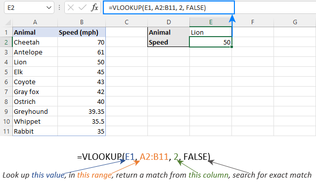
For the sake of convenience, you can type the value of interest in some cell, say E1, replace the "hardcoded" text with the cell reference, and get the formula to look up any value you input in E1:
=VLOOKUP(E1, A2:B11, 2, FALSE)
Does anything remain unclear? Then try looking at it this way:
How to do a Vlookup in Excel
When using VLOOKUP formulas in real-life worksheets, the main rule of thumb is this: lock table array with absolute cell references (like $A$2:$C$11) to prevent it from changing when copying a formula to other cells.
The lookup value in most cases should be a relative reference (like E2) or you can lock only the column coordinate ($E2). When the formula gets copied down the column, the reference will adjust automatically for each row.
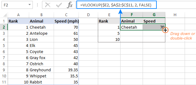
To see how it works in practice, please consider the following example. To our sample table, we have added one more column that ranks the animals by speed (column A) and want to find the 1st, 5th and 10th fastest sprinter in the world. For this, enter the lookup ranks in some cells (E2:E4 in the screenshot below), and use the following formulas:
To pull the animal names from column B:
=VLOOKUP($E2, $A$2:$C$11, 2, FALSE)
To extract speed from column C:
=VLOOKUP($E2, $A$2:$C$11, 3, FALSE)
Enter the above formulas in cells F2 and G2, select those cells, and drag the formulas to the below rows:
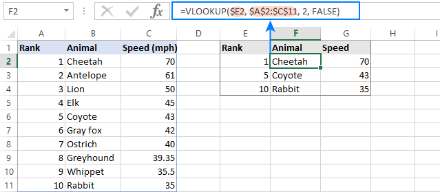
If you investigate the formula in a lower row, you will notice that the lookup value reference has adjusted for that specific row, while the table array is unchanged:
Below, you will have a few more useful tips that will save you a lot of headache and troubleshooting time.
Excel VLOOKUP - 5 things to remember!
- The VLOOKUP function cannot look at its left. It always searches in the leftmost column of the table array and returns a value from a column to the right. If you need to pull values from left, use the INDEX MATCH (or INDEX XMATCH in Excel 365) combination that can does not care about the positioning of the lookup and return columns.
- The VLOOKUP function is case-insensitive, meaning that uppercase and lowercase characters are treated as equivalent. To distinguish the letter case, use case sensitive VLOOKUP formulas.
- Remember about the importance of the last parameter. Use TRUE for approximate match and FALSE for exact match. For full details, please see VLOOKUP TRUE vs. FALSE.
- When searching for approximate match, make sure the data in the lookup column is sorted in ascending order.
- If the lookup value is not found, a #N/A error is returned. For information about other errors, please see Why Excel VLOOKUP is not working.
Excel VLOOKUP examples
I hope vertical lookup is starting to look a bit more familiar to you. To strengthen your knowledge, let's build a few more VLOOKUP formulas.
How to Vlookup from another sheet in Excel
In practice, the Excel VLOOKUP function is rarely used with data in the same worksheet. Most often you will have to pull matching data from a different worksheet.
To Vlookup from a different Excel sheet, put the worksheet's name followed by an exclamation mark in the table_array argument before the range reference. For example, to search in the range A2:B10 on Sheet2, use this formula:
=VLOOKUP("Product1", Sheet2!A2:B10, 2)
Of course, you don't have to type the sheet's name manually. Simply, start typing the formula and when it comes to the table_array argument, switch to the lookup worksheet and select the range using the mouse.
For instance, this is how you can look up the A2 value in the range A2:A9 on the Prices worksheet and return a matching value from column C:
=VLOOKUP(A2, Prices!$A$2:$C$9, 3, FALSE)
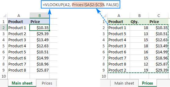
Notes:
- If the spreadsheet name contains spaces or non-alphabetical characters, it must be enclosed in single quotation marks, e.g. 'Price list'!$A$2:$C$9.
- In case you use a VLOOKUP formula for multiple cells, remember to lock table_array with the $ sign, like $A$2:$C$9.
How to Vlookup from another workbook in Excel
To Vlookup from a different Excel workbook, put the workbook's name enclosed in square brackets before the worksheet's name.
For example, here's the formula to look up the A2 value on the sheet named Prices in the Price_List.xlsx workbook:
=VLOOKUP(A2, [Price_List.xlsx]Prices!$A$2:$C$9, 3, FALSE)
If either a workbook name or worksheet name contains spaces or non-alphabetical characters, you should enclose them in single quotes like this:
=VLOOKUP(A2, '[Price List.xlsx]Prices'!$A$2:$C$9, 3, FALSE)
The easiest way to make a VLOOKUP formula that refers to a different workbook is this:
- Open both files.
- Start typing your formula, switch to the other workbook, and select the table array using the mouse.
- Enter the remaining arguments and press the Enter key to complete your formula.
The result will look somewhat like the screenshot below:
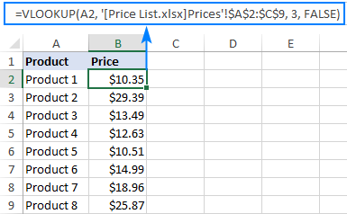
Once you close the file with your lookup table, the VLOOKUP formula will continue working, but it will now display the full path for the closed workbook:

For more information, please see How to refer to another Excel sheet or workbook.
How to Vlookup from a named range in another sheet
In case you plan to use the same lookup range in many formulas, you can create a named range for it and type the name directly in the table_array argument.
To create a named range, simply select the cells and type the name you want in the Name box to the left of the Formula bar. For the detailed steps, please see How to name a range in Excel.
For this example, we gave the name Prices_2020 to the data cells (A2:C9) in the lookup sheet and get this compact formula:
=VLOOKUP(A2, Prices_2020, 3, FALSE)
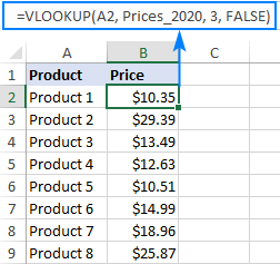
Most names in Excel apply to the entire workbook, so you don't need to specify the worksheet's name when using named ranges.
If the named range is in another workbook, put the workbook's name before the range name, for example:
=VLOOKUP(A2, 'Price List.xlsx'!Prices_2020, 3, FALSE)
Such formulas are far more understandable, aren't they? Besides, using named ranges can be a good alternative to absolute references. Since a named range doesn't change, you can be sure that your table array will remain locked no matter where the formula is moved or copied.
If you have converted your lookup range into a fully-functional Excel table, then you can do a Vlookup based on the table name, e.g. Price_table in the below formula:
=VLOOKUP(A2, Price_table, 3, FALSE)
Table references, also called structured references, are resilient and immune to many data manipulations. For instance, you can remove or add new rows to your lookup table without worrying about updating the references.
Using wildcards in VLOOKUP formula
Like many other formulas, the Excel VLOOKUP function accepts the following wildcard characters:
- Question mark (?) to match any single character.
- Asterisk (*) to match any sequence of characters.
Wildcards prove really useful in many situations:
- When you do not remember the exact text you are looking for.
- When you are looking for a text string that is part of the cell contents.
- When a lookup column contains leading or trailing spaces. In that case, you may rack your brain trying to figure out why a normal formula does not work.
Example 1. Look up text starting or ending with certain characters
Suppose you want to find a certain customer in the below database. You do not remember the surname, but you are confident that it starts with "ack".
To return the last name from column A, use the following Vlookup wildcard formula:
=VLOOKUP("ack*", $A$2:$B$10, 1, FALSE)
To retrieve the license key from column B, use this one (the difference is only in the column index number):
=VLOOKUP("ack*", $A$2:$B$10, 2, FALSE)
You can also enter the known part of the name in some cell, say E1, and combine the wildcard character with the cell reference:
=VLOOKUP(E1&"*", $A$2:$B$10, 1, FALSE)
The below screenshot shows the results:
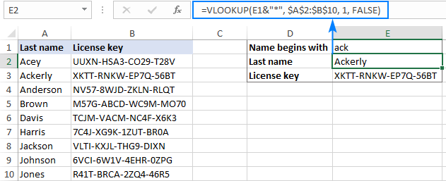
Below are a few more VLOOKUP formulas with wildcards.
Find the last name ending with "son":
=VLOOKUP("*son", $A$2:$B$10, 1, FALSE)
Get the name that starts with "joh" and ends with "son":
=VLOOKUP("joh*son", $A$2:$B$10, 1, FALSE)
Pull a 5-character last name:
=VLOOKUP("?????", $A$2:$B$10, 1, FALSE)
Example 2. VLOOKUP wildcard based on cell value
From the previous example, you already know that it is possible to concatenate an ampersand (&) and a cell reference to make a lookup string. To find a value that contains a given character(s) in any position, put an ampersand before and after the cell reference.
Let's say, you wish to get a name corresponding to a certain license key, but you don't know the whole key, only a few characters. With the keys in column A, names in column B, and part of the target key in E1, you can do a wildcard Vlookup in this way:
Extract the key:
=VLOOKUP("*"&E1&"*", $A$2:$B$10, 1, FALSE)
Extract the name:
=VLOOKUP("*"&E1&"*", $A$2:$B$10, 2, FALSE)

Notes:
- For a wildcard VLOOKUP formula to work correctly, use an exact match (FALSE is the last argument).
- If more than one match is found, the first one is returned.
VLOOKUP TRUE vs FALSE
And now, it's time to take a closer look at the last argument of the Excel VLOOKUP function. Though optional, the range_lookup parameter is highly important. Depending on whether you choose TRUE or FALSE, your formula may yield different results.
Excel VLOOKUP exact match (FALSE)
If range_lookup is set to FALSE, a Vlookup formula searches for a value that is exactly equal to the lookup value. If two or more matches are found, the 1st one is returned. If an exact match is not found, the #N/A error occurs.
Excel VLOOKUP approximate match (TRUE)
If range_lookup is set to TRUE or omitted (default), the formula looks up the closest match. More precisely, it searches for an exact match first, and if an exact match is not found, looks for the next largest value that is less than the lookup value.
An approximate match Vlookup works with the following caveats:
- The lookup column must be sorted in ascending order, from smallest to largest, otherwise a correct value may not be found.
- If the lookup value is smaller than the smallest value in the lookup array, a #N/A error is returned.
The following examples will help you better understand the difference between an exact match and approximate match Vlookup and when each formula is best to be used.
Example 1. How to do an exact match Vlookup
To look up an exact match, just put FALSE in the last argument.
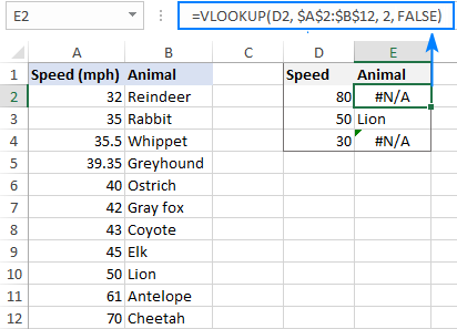
For this example, let's take the animal speed table, swap the columns, and try to find the animals that can run 80, 50 and 30 miles per hour. With the lookup values in D2, D3 and D4, enter the below formula in E2, and then copy it down to two more cells:
=VLOOKUP(D2, $A$2:$B$12, 2, FALSE)
As you can see, the formula returns "Lion" in E3 because they run exactly 50 per hour. For the other two lookup values an exact match is not found, and #N/A errors appear.
Example 2. How to Vlookup for approximate match
To look up an approximate match, there are two essential things you need to do:
- Sort the first column of table_array from smallest to largest.
- Use TRUE for the range_lookup argument or omit it.
Sorting the lookup column is very important because the VLOOKUP function stops searching as soon as it finds a close match smaller than the lookup value. If the data is not sorted properly, you may end up having really strange results or a bunch of #N/A errors.
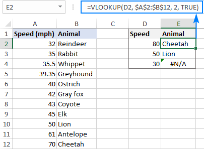
For our sample data, an approximate match Vlookup formula goes as follows:
=VLOOKUP(D2, $A$2:$B$12, 2, TRUE)
And returns the following results:
- For a lookup value of "80", "Cheetah" is returned because its speed (70) is the closest match that is smaller than the lookup value.
- For a lookup value of "50", an exact match is returned (Lion).
- For a lookup value of "30", a #N/A error is returned because the lookup value is less than the smallest value in the lookup column.
Video: How to VLOOKUP in Excel
Step-by-step guidance on how to create and use a VLOOKUP formula in Excel.
Special tools to Vlookup in Excel
Undoubtedly, VLOOKUP is one of the most powerful and useful Excel functions, but it's also one of the most confusing ones. To make the learning curve less steep and experience more enjoyable, we included a couple of time-saving tools in our Ultimate Suite for Excel.
VLOOKUP Wizard - easy way to write complex formulas
The interactive VLOOKUP Wizard will walk you through the configuration options to build a perfect formula for the criteria you specify. Depending on your data structure, it will use the standard VLOOKUP function or an INDEX MATCH formula that can pull values from left.
To get your custom-tailored formula, this is what you need to do:
- Run the VLOOKUP Wizard.
- Choose your main table and lookup table.
- Specify the following columns (in many cases they are picked automatically):
- Key column - the column in your main table containing the values to look up.
- Lookup column - the column to look up against.
- Return column - the column from which to retrieve values.
- Click the Insert button.
The following examples show the wizard in action.
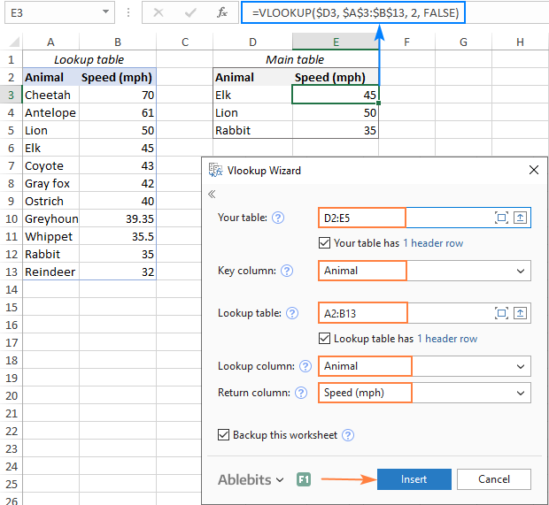
Standard Vlookup
When the lookup column (Animal) is the leftmost column in the lookup table, a normal VLOOKUP formula for exact match is inserted:
Vlookup to the left
When the lookup column (Animal) is on the right side of the return column (Speed), the wizard inserts an INDEX MATCH formula to Vlookup right to left:
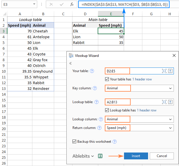
Extra bonus! Due to the clever use of cells references, the formulas can be copied or moved to any column, without you having to update the references.
Merge Two Tables - formula-free alternative to Excel VLOOKUP
If your Excel files are enormously large and complex, the project's deadline is imminent, and you are looking for someone who can lend you a helping hand, try out the Merge Tables Wizard.
This tool is our visual and stress-free alternative to Excel's VLOOKUP function, which works this way:
- Select your main table.
- Select the lookup table.
- Choose one or several common columns as the unique identifier(s).
- Specify which columns to update.
- Optionally, choose the columns to add.
- Allow the Merge Tables Wizard a few seconds for processing… and enjoy the results :)

That's how to use VLOOKUP in Excel at the basic level. In the next part of our tutorial, we will discuss advanced VLOOKUP examples that will teach you how to Vlookup multiple criteria, return all matches or Nth occurrence, perform double Vlookup, look up across multiple sheets with a single formula, and more. I thank you for reading and hope to see you next week!
Available downloads
Excel VLOOKUP formula examples (.xlsx file)
Ultimate Suite 14-day fully-functional version (.exe file)
 by
by
229 comments
Hello,
What is the formula to compare the exact numbers in two sheets.
I would like to compare the data in two sheets and find out a exact matches / numbers.
Eg: In Sheet1 : Column A: 2352,25897,25666,29981
In Sheet2 : Column A: 29981,23514,2352,25555,25369
Thanks,
Sanju
Hello,
I'm using the lookup function and it's behaving oddly: it won't find any text string in one column that starts with P to Z. I have no idea about this! Thanks!
Hello Stephen,
Please see the following blog post that describes practically all possible issues with the VLOOKUP function:
https://www.ablebits.com/office-addins-blog/excel-vlookup-not-working/
If none of the solutions help, please send your Excel file to support@ablebits.com and include the link to this blog post and your comment number.
We'll do our best to assist you.
In doing the vlookup here is my fomula,=IF(ISERROR(VLOOKUP(D2,F2:F80833, 1, FALSE)),FALSE,TRUE) and I am trying to repeat the formula where D2 changes on the next cell to D3 and so forth to D92563 but I do not want the second portion of my formula F2:F80833 to change. I cannot click and drag because it will change the 2nd portion of my formula to match. What do I do to copy portions of the formula?
Hello Jerry,
You can add a dollar sign before the column and row references to make them absolute:
=IF(ISERROR(VLOOKUP(D2,$F$2:$F$80833, 1, FALSE)),FALSE,TRUE)
This will keep the range invariable when you copy the formula.
Why while using vlookup function #NA# results if the value does exist
Hi Monika,
Because it is designed by Microsoft this way. If you'd rather display a blank cell or some message when a lookup value is not found, you can enclose your Vlookup formula in the IFERROR function:
=IFERROR(vlookup(), "")
You can find an example of a real-life formula with the detailed explanation and screenshots in this tutorial: Why Excel VLOOKUP is not working
how did four sheet use a Vlookup why Formulas
Hello Hanmant,
Could you please clarify your question? If you are not sure if the VLOOKUP function does what you need, please describe your task. We'll do our best to assist you.
have two columns in a single work sheet and I want to use VLOOKUP formula (I do not want to use MATCH Formula) to compare these two columns each other and get an output of Matching Items.
1202 16003
1206 16010
16003 21307EXQW33
16010 21307EXQW33C3
21307EXQW33 1202
21307EXQW33C3 1206
22206EXW33 22210EXQW33
22210EXQW33 22215EXW33KC3
22215EXW33KC3 22206EXW33
I want to get :
1> Compare and give teh matching output.
Hello Anil,
You can use VLOOKUP formula, e.g. =VLOOKUP(A2,$B$2:$B$11,1,FALSE), but it will simply display the value if it occurs in your lookup column.
If your task is to see whether or not value in column A is repeated in column B, you can use the following formula:
=IF(ISERROR(VLOOKUP(A2,$B$2:$B$11,1,FALSE))=FALSE,"duplicate","Unique")
I hope this helps.
I ve this formula =VLOOKUP(D7,INDIRECT(""&G9&"!B7:AL32"),2,0). I want add hyperlink in this formula as a vlookup result how?
Hello Pravin,
Could you please describe your task in more detail? Are you trying to add a hyperlink with the lookup value as the "friendly name"? If possible, please send a test spreadsheet with the description of your data and the expected results to support@ablebits.com.
We'll do our best to assist you.
Hi, what should I should I input if the look_up value is a text. Thanks
Hi Jo,
You should input that text in double quotes, e.g.
=VLOOKUP("apples", A2:B20, 2)
hello excel i am working in a school i have to maintain daily register of cash collection and total amount is to be divided into different heads like tution fee exam fee bus fee i want that formula that itself divide that amount into different heads of different class
Hello Sameer,
Could you please send a test worksheet to support@ablebits.com and describe your task and the expected result in more detail? We'll do our best to assist you.
No doubt your site is very helpful, especially for beginners like me.
Thanks very helpful lession
My spreadsheet has a field containing a drop-down list for Part category. In the field next to it, I have a drop-down list for SubCategory. When I select a sepecific Part category, I would like the SubCategory pull-down list to ONLY contain the pertinent subcategories for the Part Category selected, not everything in the SubCategory list. My SubCategory tab containing the items for the drop-down list holds the Subcategories in one column, and the Category to which the SubCategory is pertinent in the adjacent column.
What is the best way to have ONLY the Subcategories for a specific Part Category to be displayed in the SubCategory drop-down list without having to make a separate set of lists for each part category?
Hello Chuck,
When creating a drop-down list for the SubCategories, go to Data -> Data Validation, select List and instead of entering the list name in the "Source" field, use the INDIRECT function to reference the value in the cell with the Part Category, e.g.:
=INDIRECT($H2)
You will need to have named ranges for categories and subcategories. The name of the range with Subcategories must coincide with the value selected as the part category. E.g. If you select "Subcategory1" as your Part category in cell H2, then you'll get the "Subcategory1" drop-down list in I2. If this doesn't help, please send a test spreadsheet to support@ablebits.com, we'll do our best to assist you.
Awesome! I think this should be added to your page on troubleshooting why the VLOOKUP doesn't work. Can't believe they set the default to approximate match.
THANKS!!!!
thanks man, i was going nuts over this. ur solution helped. just needed to click false on range lookup
Lots of learning while reading the Q & A.. *clap*
WOW!
Hello,
I have two sheets one sheet has entire data with values & another sheet has selected items which doesn't have any values. i want put the values which selected items.
For Example:If clothes value is $ 10 in existing sheet. and selected items felter with clothes and i want to put the value 10. how can i do this by using vlookup or any other formula?
Hello Imran,
Could you please send a test worksheet to support@ablebits.com and point us to one row with the expected result? We'll do our best to assist you.
Hi Svetlana,
In excel , I have selected a cell(b1) and made it a dropdown list.
Also i have created a table(Table2) AT Sheet1!$H$6:$J$8 -> This table contains information like type(H) tool(I) and version(J).
Note that version column contains dropdown list mentioning version no.s present.
Also note that the list in b1 is pointing to table_column(H) (eg. by using data validation src=table2)
Now my requirement is when i select a value at b1 from the list, then a new Field has to be entered in a2 with the values of the table_columns (I & J)
I have got partial answer by using =VLOOKUP(B1,Table2,3,0), but as i said its not giving the drop down list in a2 its just giving the value same as in table.. I want drop down list in a2 by the above formula
Clear, step by step and with examples. An excellent tutorial!
I have two Workbooks that I need combined. On the first workbook (Workbook 1) I pull data from a website that has about 500 names in Column A (along with other data corresponding to the person in the row). I have another Workbook (Workbook 2) that I have different comments (Column E) on the person in Column A. Am I able to pull the new data for Workbook 1 and add the comments from my old Workbook 2 to the first blank Column (Column I)? Every time I pull the new info on Workbook 1 some of the names change so I can't just cut and paste the entire column.
Hello Matt,
This is exactly what the VLOOKUP function does. Enter the formula into column I of workbook 1 to pull the corresponding comments from Workbook2, e.g.:
=VLOOKUP($A2,[Workbook2.xlsx]Sheet5!A2:E26,5,FALSE)
I have two values Male and female. I want to create a fomular that adds either of them. Say everytime I add M, it aggregates it to 1, 2, 3, 4, 5 to nth value. can someone help.
Thank you.
Hi,
May i know how to lock vlooklup target to different workbook.
Example:Its alwasy lock to Numbers.xlsx
=VLOOKUP(40,[Numbers.xlsx]Sheet2!A2:B15,2)
Hi Jemi,
Simply change the workbook name [Numbers.xlsx] and the sheet name Sheet2! to different names. If you do Vlookup within the same sheet, you don't need to specify either the workbook or worksheet name.
Hi Svetlana,
Thank you for you replay.There is 2 different Workbook.
Here the condition in Workbook1
=VLOOKUP(M7,[ECA_partslist.xlsx]vlookup!A1:AF15,2,FALSE)
Workbook2: ECA_partlist.xlsx, There is 2 tab sheet in this book name 'PartList' & ' vlookup'
The situation is,the condition will auto add path if the ECA_partslist.xlsx open in different location with Workbook1 for example:
=VLOOKUP(M7,'Z:\Project\SO201504081701 Willowglen\[ECA_partslist.xlsx]vlookup'!A1:AF15,2,FALSE)
I add abit here,
Its happend when I save the Workbook1 in different location with Workbook 2(ECA_partlist.xlsx. Not only the vlookoup path effected but 'Name Manager' refer to also will add the path.
Hi, I have this problem
Pers # Surname FullNames Job Titles
k15126 Abure Data Moses Security Officer
in another sheet2 i have
Pers # Surname FullNames Job Title Start Date
k15126 Abure Data Moses Security Officer 2015-10-02
I want to vlookup start dates in sheet 2 to include in sheet1 to match their pers # Surname FullName and Jobe Titles
Help
how to use vlookup for sheet 1 to worksheet same row with one colom.
Hai
I have a problem.
I have two work books. One shows part no and price in different columns. Another work book where I prepare quotations. Is there any formula, so that when I enter the part no in the quotation work sheet, price will be automatically come in the price column of the quotation work sheet
Hi
How can I use vlookup formula using with OR function?
I have more than 40000 line items from which I have to match the data using vlookup and in some cases cells having error eventhough the data is lying in main table.
Pls help me.
CA Nishit Shah
My Query
I have 12 sheets in a work book. I wanted to consolidate all the entries in all the work sheet in one sheet through vlookup.
Please reply with result.
Regards
dhanuskodi
My query:
I have two column A & B each had got 10000 entries , A is original and B is typed in. I want to find error in B by comparing both column A & B
Entries e.g. 1-721-95-43
Please reply with result oriented solution
Regards,
Afzaal
When I type in a vlookup formula, the cell shows the formula not the result?
What am I doing wrong here?
Hello Tim,
Please make sure you enter the equals sign before the formula, e.g.
=VLOOKUP(40,Sheet2!A2:B15,2)
Tim,
Most likely you have inadvertently activated the Show Formulas mode in your worksheet. To turn it off, press the CTRL+` shortcut. If it's not the case, check out other possible reasons and fixes: Why is Excel showing formula, not result?
I have two workbooks. Workbook "A" has been completed and now contains questions and the responses of the Interviewee. Workbook "B" contains a number of additional cells which are the bases of the final report to management. I constructed "VLOOKUP" code to pull questions entered in Workbook "A" and pace them in the appropriate column in Workbook "B". What I want is this to happen only once when Workbook "B" is opened. Can I do this using just formulas or do I need to use VBA code?
Hi! I have a list of weeks that gets refreshed periodically, like:
2015|05 (2)
2015|06 (3)
2015|07 (4)
2015|08 (5)
2015|09 (6)
and so on. And I want to make a vlookup reference to them, but on my other table the dates get refreshed with a little difference, like:
2015|05 (11)
2015|06 (12)
2015|07 (13)
How can I make the reference work? Because I tried to make the range_lookup cell TRUE (an approximate match), but then the result is not correct.
Thanks a lot!
For problem 2 of the vlookup examples how would one go about figuring that out? I understand it's something like vlookup("Jamie"&"Jackie,$B$5:$E$17... but I'm lost from there. How do you compare the two values to come out with the higher value?
Hi. Hope you well.im struggling to get resolve the problem with my vlookup. It continues show #NA. Can i please e-mail the workbook to you? I urgently need help and need to know how to avoid this in problem in the future. Many thanks.
Hi Chica,
Our season holidays have already started, that is why we won't be able to look at your sheet until Jan 2015, I am really sorry.
In the meantime, please have a look at the following article that explains all possible errors with VLOOKUP and the ways to fix them:
https://www.ablebits.com/office-addins-blog/excel-vlookup-not-working/
Hi,
I have an issue where in sheet 1 I have different no like
1
2
3
4
5
6
and I have to put data from 2 different sheet which have
2
4
6
in sheet 2
1
3
5
in sheet 3
so what single formula we can use so that data can be come in sheet 1 from sheet 2 and 3
pls suggest
hi i am unable to understand this and i am new to this vlookup can you help me out of this problem. ple....Svetlana Cheusheva
Thanks very very very much for your good information ms excel. I want to learn form u more and more from u thanks and regards sham india please send more tips on my email
Hi
I have a date in dd/mm/yyyy HH:MM:SS (26/11/2014 01:51:08)formatt, I want to use a wildcard vlookup. I tried =vlookup("26/11/2014*", etc etc.
But no joy, can you help?
Thanks
Matt
2 coloum common vlookup actually I need to compare with booking with stock what I am having. Kindly help me. eg : In sheet1 bookings & in another sheet2 stock. model wise colour is common for both sheet. I need to arrive against stock the booking of the customer name.
Please help me
surekha
Hello Surekha,
The solution for this task is described in the following articles, hopefully you will find them helpful:
https://www.ablebits.com/office-addins-blog/vlookup-formula-examples/#vlookup-multiple-criteria
https://www.ablebits.com/office-addins-blog/excel-index-match-function-vlookup/#lookup-multiple-criteria
Hello Rosie,
Because Excel VLOOKUP cannot look at its left, it cannot return a value from a column located to the left of the lookup column. In this can you can use an INDEX / MATCH formula like this:
=INDEX(NOMINA!E:E,MATCH(B8,NOMINA!H:H,0))
Where B8 is the lookup value, column E in NOMINA sheet is the lookup column and column H in the NOMINA sheet is the return column.
For more details about using INDEX MATCH as a more flexible alternative to VLOOKUP, please see this tutorial:
https://www.ablebits.com/office-addins-blog/excel-index-match-function-vlookup/
Actually the returned is column E in the NOMINA sheet and column H is the lookup column
Hi, first of all, thanks a lot for giving us these tips and explanations, they are very useful.
What if I want to find a value that is not on the first column? On the Speed/Animal example, what if I want my Vlookup formula to find the value Antelope so it will show me that animal's speed instead of doing it the other way around.
I have 2 different sheets, I want to be able to create a Vlookup formula on sheet #1 that will allow me to match a value that is on the H column of the 2nd sheet and I want it to give me the value on the column E of the same sheet (I cannot change what's on the 2nd sheet). I tried something like =VLOOKUP(B8,NOMINA!A:H,5,FALSE), but it doesn't work.
Thank for ur introdution of vlookup
Thank you for the tutorial on using Vlookup with a separate workbook!
I had tried it, it is EXCELLENT
Thank you.
How I use the VLOOKUP formula in the situation below,
for example;
5 4 4 3 4 4 4 5 5 4 5 2
the total number of 5 in this row is 4, how can I formula it so that I can use sum up a specified number in a row of more than 100 numbers or more?
Thank you.
Hello Angel,
Please use the SUMIF and COUNTIF functions:
=countif(A2:A100, 5)
=sumif(A2:A100, 5)
Where A2:A100 is the column with numbers, 5 is the number you want to count / sum.
You can find more information about the COUNTIF function in this article:
https://www.ablebits.com/office-addins-blog/excel-countif-function-examples/
Thanks, excellent example
The Most Important VLOOKUP function in MS Office (Excel). You can big database in find one person of the result. Thank You
EXCELLENT
WANT TO LEARN MORE FROM YOU..Its too good
With best regards
UDAY
Waiting for ur suggestion.
Hello Madhu,
Thank you for your workbook. I am sorry, we are overloaded with work at the moment. We'll try to look at your task as soon as we can.
Hi Madam
i sent a mail ur mentioned mail id please find the mail .
Hi
Thanks for your valuable feedback.
Finding solution in a work sheet row's a1 b1 c1 d1..... Contained descriptions and same column have many part numbers. If a cell reference part number by matching index. description will be auto generated. please let me know if any formula is there?
Hi Madhu,
I think it will be easier for me to write the correct formula if I can see your sample data. If you can send me your workbook at support@ablebits.com and give an example of the expected result, I will try to help.
Hi Svetlana,
May I send you sample data sheet for vlookup formula.
Hi Svetlana,
Please help me I want to find value from 2 pairs of different columns in same sheet by inserting Vlookup formula.
Please suggest inputs.
regards,
Arjun Yadav
hi svetlana nice working excel working and as only work
i am freind and frankily
More vlookup function details
You can find more information about various aspects of Excel Vlookup in the links posted at the end of this tutorial.