Is your VLOOKUP pulling wrong data or you cannot get it to work at all? This tutorial shows how you can quickly fix common VLOOKUP errors and overcome its main limitations.
In a few earlier articles, we explored different aspects of the Excel VLOOKUP function. If you have been following us closely, by now you should be an expert in this area :)
However, it's not without reason that many Excel specialists consider VLOOKUP to be one of the most intricate Excel functions. It has a ton of limitations, which are the source of various problems and errors.

In this article, you will find simple explanations of the main causes of VLOOKUP errors such as #N/A, #NAME and #VALUE, as well as their solutions and fixes. We will start with the most obvious reasons why VLOOKUP is not working, so it might be a good idea to check out the below troubleshooting steps in order.
Fixing #N/A error in VLOOKUP
In VLOOKUP formulas, the #N/A error message (meaning "not available") is displayed when Excel cannot find a lookup value. There can be several reasons why that may happen.
1. The lookup value is misspelt
It's always a good idea to check the most obvious thing first : ) Misprints frequently occur when you are working with really large data sets consisting of thousands of rows, or when a lookup value is typed directly in the formula.
2. #N/A in approximate match VLOOKUP
If your formula looks up the closest match, (range_lookup argument set to TRUE or omitted), the #N/A error can appear in two cases:
- The lookup value is smaller than the smallest value in the lookup array.
- The lookup column is not sorted in ascending order.
3. #N/A in exact match VLOOKUP
If you are searching for exact match (range_lookup argument set to FALSE), the #N/A error occurs when a value exactly equal to the lookup value is not found. For more information, see VLOOKUP exact match vs. approximate match.
4. The lookup column is not the leftmost column of the table array
One of the most significant limitations of Excel VLOOKUP is that it cannot look to its left. Consequently, a lookup column should always be the leftmost column in the table array. In practice, we often forget about this and end up with #N/A errors.
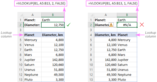
Solution: If it is not possible to restructure your data so that the lookup column is the left-most column, you can use the INDEX and MATCH functions together as an alternative to VLOOKUP. Here's a formula example: INDEX MATCH formula to look up values to left.
5. Numbers are formatted as text
Another common source #N/A errors in VLOOKUP formulas is numbers formatted as text, either in the main or lookup table.
This usually occurs when you import data from some external database or if you've typed an apostrophe before a number to show leading zeros.
Here are the most obvious indicators of numbers formatted as text:
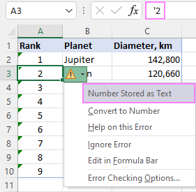
Solution: Select all the problematic numbers, click on the error icon and choose Convert to Number from the context menu. For more information, please see How to convert text to number in Excel.
6. Leading or trailing spaces
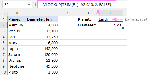
This is the least obvious cause of the VLOOKUP #N/A error because a human eye can hardly spot those extra spaces, especially when working with big datasets where most of the entries are below the scroll.
Solution 1: Extra spaces in the lookup value
To ensure the correct work of your VLOOKUP formula, wrap the lookup value in the TRIM function:
=VLOOKUP(TRIM(E1), A2:C10, 2, FALSE)
Solution 2: Extra spaces in the lookup column
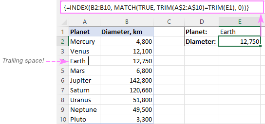
If extra spaces occur in the lookup column, there is no easy way to avoid #N/A errors in VLOOKUP. Instead, you can use a combination of INDEX, MATCH and TRIM functions as an array formula:
=INDEX(B2:B10, MATCH(TRUE, TRIM(A$2:A$10)=TRIM(E1), 0))
Since this is an array formula, don't forget to press Ctrl + Shift + Enter to properly complete it (in Excel 365 and Excel 2021 where arrays are native, this also works as a regular formula).
Tip. A quick alternative is running the Trim Spaces tool that will eliminate excess spaces both in the lookup and main tables in seconds, making your VLOOKUP formulas error-free.
#VALUE! error in VLOOKUP formulas
In general, Microsoft Excel displays the #VALUE! error if a value used in the formula is of a wrong data type. In respect to VLOOKUP, there are three common sources of the VALUE! error.
1. Lookup value exceeds 255 characters
Please be aware that VLOOKUP cannot look up values containing more than 255 characters. If your lookup values exceed this limit, a #VALUE! error will be displayed:

Solution: Use an INDEX MATCH formula instead. In our case, this formula works perfectly:
=INDEX(B2:B7, MATCH(TRUE, INDEX(A2:A7= E1, 0), 0))

2. Full path to the lookup workbook is not supplied
If you are pulling data from another workbook, you have to include the full path to it. More precisely, you have to enclose the workbook's name including the extension in [square brackets] and specify the sheet's name followed by the exclamation mark. If the workbook name or sheet name, or both, contain spaces or any non-alphabetical characters, the path must be enclosed in single quotation marks.
Here's the structure of the table_array argument to Vlookup from another workbook:
'[workbook name]sheet name'!range
A real formula might look similar to this:
=VLOOKUP($A$2,'[New Prices.xls]Sheet1'!$B:$D, 3, FALSE)
The above formula will search for the value of A2 in column B of Sheet1 in the New Prices workbook, and return a matching value from column D.
If any element of the path is missing, your VLOOKUP formula won't work and return the #VALUE error (unless the lookup workbook is currently open).
For more information, please see:
3. The col_index_num argument is less than 1
It's hard to imagine a situation when someone intentionally enter a number less than 1 to specify the column to return values from. But it may happen if this argument is returned by some other function nested in your VLOOKUP formula.
So, if the col_index_num argument is than 1, your formula will return the #VALUE! error too.
If col_index_num is greater than the number of the columns in the table array, VLOOKUP produces the #REF! error.
Solving VLOOKUP #NAME error
This is the easiest case - the #NAME? error appears if you've accidentally misspelled the function's name.
The solution is obvious - check the spelling :)
The main causes of errors in Excel VLOOKUP
Apart from having a fairly complicated syntax, VLOOKUP has arguably more limitations than any other Excel function. Because of these limitations, a seemingly correct formula may often deliver results different from what you expected. Below you will find solutions for a few typical scenarios when VLOOKUP fails.
VLOOKUP is case-insensitive
The VLOOKUP function does not distinguish the letter case and teats lowercase and uppercase characters as identical.
Solution: Use VLOOKUP, XLOOKUP or INDEX MATCH in combination with the EXACT function that can match text case. You can find the detailed explanations and formula examples in this tutorial: 5 ways to do a case-sensitive Vlookup in Excel.
A new column was inserted or removed from the table
Regrettably, VLOOKUP formulas stop working every time when a new column is deleted from or added to the lookup table. This happens because the syntax of the VLOOKUP function requires defining the index number of the return column. When a new column is added to/removed from the table array, obviously that index number changes.
Solution: The INDEX MATCH formula comes to the rescue again : ) With INDEX MATCH, you specify the lookup and return ranges separately, so you are free to delete or insert as many columns as you want without worrying about updating every associated formula.
Cell references change when copying the formula to other cells
The heading gives an exhaustive explanation of the problem, right?
Solution: Always use absolute references (with the $ sign) for the table_array argument, e.g. $A$2:$C$100 or $A:$C. You can quickly switch between different reference types by pressing the F4 key.
VLOOKUP returns the first found value
As you already know, Excel VLOOKUP returns the first value it finds. However, you can force it to bring the 2nd, 3rd, 4th or any other occurrence you want. There is also a way to get the last match or all found matches.
Solutions: Formula examples are available here:
Why does my VLOOKUP work for some cells but not others?
When your VLOOKUP formula returns the correct data I some cells and #N/A errors in others, there can be a few possible reasons why that happens.
1. The table array is not locked
Suppose you have this formula in row 2 (say in E2), which works nicely:
=VLOOKUP(D2, A2:B10, 2, FALSE)
When copied to row 3, the formula changes to:
=VLOOKUP(D3, A3:B11, 2, FALSE)
Because a relative reference is used for table_array, it changes based on the relative position of the row where the formula is copied, in our case from A2:B10 to A3:B11. So, if the match is in row 2, it won't be found!
Solution: When using a VLOOKUP formula for more than one cell, always lock the table array reference with the $ sign like $A$2:$B$10.
2. Text values or data types do not match
Another common reason for VLOOKUP failure is the difference between your lookup value and a similar value in the lookup column. In some cases, the difference is so subtle that it's hard to spot visually.
Solution: When VLOOKUP is returning an #N/A error while you can clearly see the lookup value in the lookup column, and apparently both are spelt exactly the same, the first thing you need to do is to determine the root cause of the problem - the formula or the source data.
To see whether the two values are the same or different, make a direct comparison in this way:
=E1=A4
Where E1 is your lookup value and A4 is an identical value in the lookup column.
If the formula returns FALSE, that means the values differ in some way, though they look absolutely alike.
In case of numeric values, the most possible reason is numbers formatted as text.
In case of text values, most likely the problem is in excess spaces. To verify this, find out the total length of the two strings using the LEN function:
=LEN(E1)
=LEN(A4)
If the resulting numbers are different (like in the screenshot below), then you've pinpointed the culprit - extra spaces:
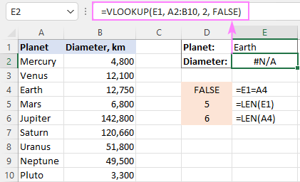
To solve the issue, either remove extra spaces or use this INDEX MATCH TRIM formula as a workaround.
Why does my VLOOKUP pull wrong data?
There could be even more reasons why your VLOOKUP returns a wrong value:
- Incorrect search mode. If you want an exact match, be sure to set the range_lookup argument to FALSE. The default is TRUE, so if you omit this argument, VLOOKUP will assume you are looking for an approximate match and search for the closest value that is smaller than the lookup value.
- The lookup column is not sorted. For approximate match VLOOKUP (range_lookup set to TRUE) to work correctly, the first column in the table array must be sorted in ascending order, from smallest to largest.
- Duplicates in the lookup column. If the lookup column contains two or more duplicate values, VLOOKUP will return the first found match, which may not be the one you expect.
- Incorrect return column. Double-check the index number in the 3rd argument :)
VLOOKUP not working between two sheets
First off, it should be noted that the common reasons of #N/A, #VALUE, and #REF errors discussed above may cause the same problems when looking up from another sheet. If it's not the case, check out the following points:
- Make sure the external reference to another sheet or a different workbook is correct.
- When doing a Vlookup from another workbook which is closed at the moment, verify that your formula contains the full path to the closed workbook.
- If VLOOKUP cannot pick a table array in another worksheet (i.e. when you highlight a range in the lookup sheet, nothing appears in the table_array argument in the formula or in the corresponding box of the formula wizard), then most likely the two sheets are open in separate instances of Excel and cannot communicate with each other. For more info, please see How to determine which Excel files are in which instance. To fix this, simply close all Excel windows, and then reopen the sheets/workbooks in the same instance (the default behavior).
How to Vlookup without errors in Excel
If you do not want to intimidate your users with standard Excel error notations, you can display your own user-friendly text instead or return a blank cell if nothing is found. This can be done by using VLOOKUP with IFERROR or IFNA function.
Catch all errors
In Excel 2007 and later, you can use the IFERROR function to check a VLOOKUP formula for errors and return your own text (or an empty string) if any error is detected.
For example:
=IFERROR(VLOOKUP(E1, A2:B10, 2, FALSE), "Oops, something went wrong")
In Excel 2003 and earlier, you can use the IF ISERROR formula for the same purpose:
=IF(ISERROR(VLOOKUP(E1, A2:B10, 2, FALSE)), "Oops, something went wrong", VLOOKUP(E1, A2:B10, 2, FALSE))
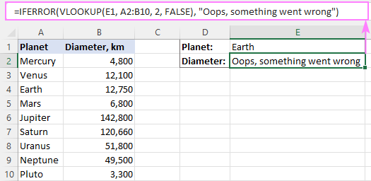
For more details, please see Using IFERROR with VLOOKUP in Excel.
Handle #N/A errors
To trap only #N/A errors ignoring all other error types, use the IFNA function (in Excel 2013 and higher) or IF ISNA formula (in all versions).
For example:
=IFNA(VLOOKUP(E1, A2:B10, 2, FALSE), "Oops, no match is found. Please try again!")
=IF(ISNA(VLOOKUP(E1, A2:B10, 2, FALSE)), "Oops, no match is found. Please try again!", VLOOKUP(E1, A2:B10, 2, FALSE))
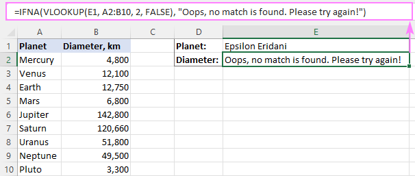
That's all for today. Hopefully, this tutorial will help you get rid of VLOOKUP errors and have your formulas working in the way you want.
How to VLOOKUP in Excel - video tutorial
 by
by
222 comments
A problem with…
"Use VLOOKUP and INDIRECT to dynamically pull data from different sheets"
=VLOOKUP($D$2,INDIRECT($D3&"_Sales"),2,FALSE)reference formula
Since my reference cell Y3 needs to be a number and my Named Ranges can start with a number (LIST15, LIST18, LIST20) I cannot get this formula to work.
=VLOOKUP($AE3,INDIRECT($Y3&"_LIST"),2,0)
I even tried to move the underscore to the right side to match the way it is in the Named Ranges and still don’t work.
=VLOOKUP($AE3,INDIRECT($Y3&"LIST_"),2,0)
I get a #REF! Error in both cases. Can anyone help?
I too facing the common error like #N/A, even after i convert the look up range in number format. kindly suggest. any other alter.
THANK YOU!!!! You just saved me. TRIM...who knew!
Hi,
My V-lookup is working, but the formula will not copying down the full column of data. For example, 100 cells of data, first cell will v-look up correctly, but the rest of the column can't be completed without repeating the v-lookup an additonal 99 times, in each cell. Does that make sense?
Any thoughts on how to fix?
Thank you.
Hello, Susan,
To help you better, we need a sample table with your data in Excel. You can email it to support@ablebits.com. Please add the link to this article and your comment number.
Had a similar issue today with a vlookup. I tried the suggestions above but nothing worked. I had to insert a value() into the field lookup value in order to conduct the search. Oddly, the field being looked up is formatted properly as well as the range it is looking at. An example:
=VLOOKUP(VALUE(A1691),DSI!$B$2:$D$769,3,FALSE)
Hello, Brian,
To help you better, we need a sample table with your data in Excel. You can email it to support@ablebits.com. Please add the link to this article and your comment number.
In certain parts of my worksheet , when i enter the vlookup function it doesnt do anything it remians as text format
Hello, Mahir,
Please make sure you enter the equal sign before adding the formula.
Hi Mahir,
Most likely it's because the format of those cells is set to "Text". Changing the cell format to "General" should fix it. If it doesn't, check out the following solutions:
Why is Excel showing a formula, not result?
Svetlana
It seems you may be able to help me. I am using Excel 2010. I created a drop-down list, and want to use VLOOKUP to complete other columns, with information in the table which I used for the drop-down list. The column for the drop-down is A.
If I make my selection from the drop-down list, nothing happens, that is my formula, e.g:=VLOOKUP($E2,Premises!$A$2:$P$101,4,FALSE) remains in the cell, with no value provided. I checked formatting of cells to make sure it is the same.
Thanks
Jacoba
Hello, Jacoba,
To understand your task better, we'd like to have a look at your data. You can email it to support@ablebits.com. Please add the link to this article and your comment number.
Thanks Svetlana
Thanks for your explanations. The problem with my vlookup was the formatting of the "search" data; formatting it as "number" solved the problem!
Hi, svetlana cheusheva
i have a query related to excel please help me
how to highlight past dates?
Hope you help me!
I think Formula is =a2<today() it is work.
I keep having my vlookup column doing this. Is there something I have to do to correct this?
=VLOOKUP(A4,October!A:A,1,0)
=VLOOKUP(A4,October!A:A,1,0)
=VLOOKUP(A4,October!A:A,1,0)
=VLOOKUP(A4,October!A:A,1,0)
=VLOOKUP(A4,October!A:A,1,0)
=VLOOKUP(A4,October!A:A,1,0)
=VLOOKUP(A4,October!A:A,1,0)
=VLOOKUP(A4,October!A:A,1,0)
Hello, Dee,
You can add a check for the found value:
=IF(ISERROR(VLOOKUP(A4,October!A:A,1,0)), "",VLOOKUP(A4,October!A:A,1,0))
WHATS with wrong (( ? )))
your utmost consideration and accommodation regarding my request would be of great help...please...
thanks
Bank Code Legend:
bpi BPI
BEGINNING BALANCE 258,581.64
ADD:
CASH DEPOSIT 270699
A/R - COLLECTIONS 530,400.00
FUND TRANSFER IN 0.00
TOTALS 801,099.00
DEDUCT:
CASH REMITTANCE 0.00
FUND TRANSFER OUT 0.00
EXPENSES 414,350.00
TOTALS 414,350.00
ENDING BALANCE TO DATE 645,330.64
good day!
i just wanna know how can i show/flash the names of clients (which is in the other sheet) who paid cash in my report? same with the client who paid their accounts receivable, which i termed "collection"?
i just want to show my boss the names of clients who paid their obligations (cash payment & collection of A/R).
i used vlookup to find the details about the "bank" (bpi) the beg balance, the cash deposit, collections etc. what i want to solve now is how can i make the names of the clients appear in my report to see in details who the clients are already based on the data i encoded. and if my boss tries to see the details of another bank, same thing i want to appear the names of clients i encoded, also..
please help me..
Thanks!!
Bank Code Legend:
bpi BPI
BEGINNING BALANCE 258,581.64
ADD:
CASH DEPOSIT 270699
A/R - COLLECTIONS 530,400.00
FUND TRANSFER IN 0.00
TOTALS 801,099.00
DEDUCT:
CASH REMITTANCE 0.00
FUND TRANSFER OUT 0.00
EXPENSES 414,350.00
TOTALS 414,350.00
ENDING BALANCE TO DATE 645,330.64
If nothing else works for number search (i.e. excessive blanks removed, data formats made the same number format) this works for me:
=vlookup(A1/1,D1:D100,2,FALSE)
Hello, this post helps to reduce time on vlookup formula, thanks
I am using a vlookup to match sales and on hand data for item numbers that contain an'*' in them. The lookup is working except for occasion where the exact value is not found, but something close is found. I am told that the wildcard '*' is the reason the formula brings back a bad result even when the vlookup uses the FALSE condition (=vlookup(A1,G1:H13000,2,FALSE. The target looks like B110015BS***GG but pulls from B110015BSR**GG. Does anyone know how to make the formula ignore the wildcard? I tried doing a find/replace, but as a wildcard, it replaced the whole string in each field..
SL No Part # Description SL No Part # Description
1 1100316 PLATE SPRING UPPE 1 1100316 #N/A
2 1100611 KEY WOODRUFF CLUTCH 2 1100342 #N/A
3 1100342 BEARING BALL 3 1100611 #N/A
4 1101008 ROLLER 4 1100818 #N/A
5 1101205 SPRING RETURN 5 1101008 #N/A
6 1180123 BALL STEEL 6 1101205 #N/A
7 1100818 WASHER BRASS 7 1180123 #N/A
__________________________________________________________________
I have checked all the columns if the
may anyone help me..? during using VLOOKUP i am facing problem, actually i have a data which have extra spaces and "" quotes etc in table array but showing simple as lookup value and obviously i am unable to get the data so pls help me..
Hello,
Excellent post! Out of all the pages I looked at to resolve this problem, yours worked. So simple and Boom!!
I was wondering if you could help me with an issue I have been having. I pull daily spreadsheets with information for employees. I have a column at the end that has my notes for each individual case. With each spreadsheet I use vlookup to transfer the most current notes from the previous day’s spreadsheet to the one I just pulled. The lookup value I use is the employee’s ID number which I always remember to convert to number. Every time I transfer the notes, the majority are correct but quite a few either populate as ‘0’, ‘#N/A’, or pull previous notes from much earlier spreadsheets. I’ve been on numerous excel forums looking for a solution and have tried many(locking the reference table array, sorting and filtering each spreadsheet the same way, etc) and none seem to work. I really appreciate any insight you can offer, correcting each spreadsheet has been a timely process that I feel I can be better spending doing other activities.
I have a list of members per month for three months and have to combine all the members of those months and mark in front of the members who were present in that perticular month. I know that it can be done by vlookup but i am not able to do it.
Please help.
I am trying to do Vlook up and it keeps on giving me #n/a
It is reading from 2 worksheets within one document;
vlookup($A3,'Venue Options'!$A:L,2,FALSE)
I have checked that my columns are in ascending order and that the cell format is set at number....
I am at a loss! I know it is difficult to see what I am doing but this is a relatively easy formula. ..
Thank you
Ali
hi,
when using the following formula =VLOOKUP(A:B,Sheet2!A:C,3,2) getting value error. pls help.
hi,
I have an assignment, using vlookup and if functions,
we cannot use the "if error" to not shown the "n/a",
what function I can use instead?
Thank you
Cris
Every time I enter a vlookup lately (I didn't use to have this problem), if returns something like =VLOOKUP(A:A,'[Restricted Detailed Employee Listing_4.14.2015_limited.xlsx]Detailed Employee Listing'!$A:$S,false,19). Please help.
How can I search the numbers with E+ in my databases of thousands records.
How can I search the numbers with E+ in my databases of thousands records
VLOOLUP not giveing correct number.
Never mind. I found the problem. There were duplicate values and it grabbed the largerst value
Hi there, I would appreciate your help.
I created a table of VLookup formulas. Worked great, but now I am trying to sum values in several rows and I get a Zero.
I would also like to average, counta and several other functions but it doesn't seem to work on the values created by VLookup.
What am I doing wrong.
Thank you so much for your help.
I am using excel 2013. when I try to do vlookup,the first row prints correct value. when I drag the formula for other columns it prints the same first value for all the other columns even if the formula is changed.
I have been using a the same Lookup in a large spreadsheet for about 4 years now. Recently I have been getting random results. In some of the cells I get the expected results but in others I just get a 0, not N/A or #Value#. I've made sure that my table is sorted in the correct order and that the data I'm looking for is in the furthest left column. I've also made sure that I have the correct range in my formula, nothing seems to help.
What could be causing this random error in my results?
Brilliant, Thanks a lot, I've searched high and low for an answer and this is the only one that I can understand and make work.
I have a spreadsheet that we update daily on one tab and we use a vlookup to update information on the main tab. The problem is that there are several client names that won't update automatically after we paste the new data. We have to clear their name each day and retype it for the vlookup to work. I have ran trim and that doesn't work. Plus my colleague cannot even update the name. The vlookup won't work at all if she updates from her excel. The names are in alphabetical order. The range is covered. THe names aren't all at the end they really have nothing in common that I can see. It seems completely random. If I retype their names the vlookup does not return the #NA but if my colleague retypes their names her Excel does not update the data. I have gone crazy trying to figure this out. Help!
We detfniiely need more smart people like you around.
The problem I frequenly run in to is the data that is being displayed by the Vlook up is both correct and incorrect. It pulls data from the wrong cell. Im pritty sure I set everything up correctly but why would it present incorrect data why not just N/A or error? In addition some of the data is represented properly. Seems sporadic on one sheet driving me nuts.
Hello,
Most likely the issue is in your data or in the way they are presented: the cells format, excess spaces, merge cells, etc.
THANK YOU!
I have an Excel 2010 document that has vlookups and other formulas. I want to share the Excel doc so that my team can update their parts and we can all be in the file. The only problem I am having is that when the document is being shared and I go to update it with new data (I am the only one on the document when I add new data) for everyone to update the vlookups stop working. What can be causing this issue?
1- Can i use vlookup formula to search for data in an excel sheet that has blank rows or columns?
2- can i build my vlookup formula on the right of the data that I need to search it?
thanks,
Tony
Hi Tony,
1) yes, the VLOOKUP formula can be used to search through blank rows/columns.
2) yes, it's up to You where You place your formula.
i what to compare my list of names, Numbers, dates in 2 sperate excel spreadsheet for each of them to finds erros.for example, i want boths spread sheet to have save figure 1245 and 1245. it if any contain 1254 then how can i corret it. example 2, i want stanley on both spreadsheet, it the ohter contain stanely, i can excel tell me the teh mistake and how can i fix it.
can anyone help me please.
Hi Sveltana,
My problem was a silly one my lookup search column wasn't sorted so it was returning a few N/A# but now it's solved. I owe you one and you got my gratitude it was really appreciated.
Thank you very much for posting this is really useful.
found the answer:
add Iferror to your formula:
=IFERROR(VLOOKUP($R2;'my database'!$E:$U;6;FALSE);" ")
This is very helpful! Thank You. Unfortunately, my VLOOKUP is still not working and I'm receiving the #N/A. I know what the issue is, but can't fix it. I am looking in a range that doesn't contain the VLOOKUP value I would like (which is ok) and I just want it to return to zero (0). Is there any way I can do that in excel?
I have been struggling for hours , you saved my life. I would have never guessed that the lookup column had to be the leftmost column of the table array..
It's just not working. I used the wizard to build the formula =VLOOKUP('Tracking In Progess'!A:A,A:A,1,'Tracking In Progess'!A:C) and it always returns #VALUE!-- I tried swapping the lookup_value and table_array and it always returns #VALUE! I've tried doing this with five different workbooks with different data. It never works. I've tried it in 2010 and 2013 and the result is always the same. I need this function -- but I hate it!
It works now that I followed Derek's comment.
Hi Chris,
It's hard to determine the cause of the problem without seeing your data. Anyway, this is not because of Excel limitations. Even in older versions of Excel, a limit to the number of items displayed in drop-down lists was 1,000. In modern versions it's 10,000.
Please help!
Disclaimer: I'm a newbiew with excel. I've created a table which has a couple hundred items which is referenced to by a vlookup. For some reason, when I am using the drop down to select an item, the drop down only shows 196 items from the table. Nothing more. The table array in the formula is correct and locked. BUt for some reason the dropdown list will only go so far. Help?
Thank you so much for your Manual uploaded
Dear,
thank you for the great information , but I review all the possible problem and I fix them , but steel #N/A! and the Looked up value is exist!!
so here is the lookup: =VLOOKUP(A2,C2:D1048534,1,FALSE)
the column A have numbers which I need to make sure if it's exist or not then give me the value for it's reference. and C, D are the array index.
and I used False because it's phone number I need the exact match.finally 1 will return the subscription date.
they both have the same type , I check with =TYPE() , also they are match I checked with A2=D3.
:) so how can I fix it?
thx
Thank you Svetlana
you are really sweet girl. what you are presenting here of useful material reflects your sweetness, kind heart and sole.
Thank you again love you and keep on.
Cheers
Jafar
Saudi Arabia
Thank you very much for your nice words, Jafar! You are too kind.
We had a problem when we upgraded to 2013.
When we sorted a table with a column containing the VLOOKUP formula
=VLOOKUP(Analysis!D3,DEPT2,2,FALSE)
The formula kept the reference to original cell that we were referring to
So, if the above formula was located on row 3, and the sort moved it to row 41, it would still reference D3, rather than D41
The table was located in the worksheet named "Analysis", so that worksheet reference was superfluous, and when we removed Analysis! from the formula, it adapted correctly to the new row following the sorting of the table.
Hello Derek,
Thank you very much for sharing this information. I've tested this behavior and got the same results.
you're so pretty