In this article, you will learn various ways to concatenate text strings, numbers and dates in Excel using the CONCATENATE function and "&" operator. We will also discuss formulas to combine individual cells, columns and ranges.
In your Excel workbooks, the data is not always structured according to your needs. Often you may want to split the content of one cell into individual cells or do the opposite - combine data from two or more columns into a single column. Common examples are joining names and address parts, combining text with a formula-driven value, displaying dates and times in the desired format, to name a few.
In this tutorial, we are going to explore various techniques of Excel string concatenation, so you can choose the method best suited for your worksheets.
What is "concatenate" in Excel?
In essence, there are two ways to combine data in Excel spreadsheets:
- Merging cells
- Concatenating cells' values
When you merge cells, you "physically" join two or more cells into a single cell. As a result, you have one larger cell that is displayed across multiple rows and/or columns.
When you concatenate cells in Excel, you combine only the contents of those cells. In other words, concatenation in Excel is the process of joining two or more values together. This method is often used to combine a few pieces of text that reside in different cells (technically, these are called text strings or simply strings) or insert a formula-calculated value in the middle of some text.
The following screenshot demonstrates the difference between these two methods:

Merging cells in Excel is the subject of a separate article, and in this tutorial, we'll discuss the two main ways to concatenate strings in Excel - by using the CONCATENATE function and the concatenation operator (&).
Excel CONCATENATE function
The CONCATENATE function in Excel is used to join different pieces of text together or combine values from several cells into one cell.
The syntax of Excel CONCATENATE is as follows:
Where text is a text string, cell reference or formula-driven value.
The CONCATENATE function is supported in all versions of Excel 365 - 2007.
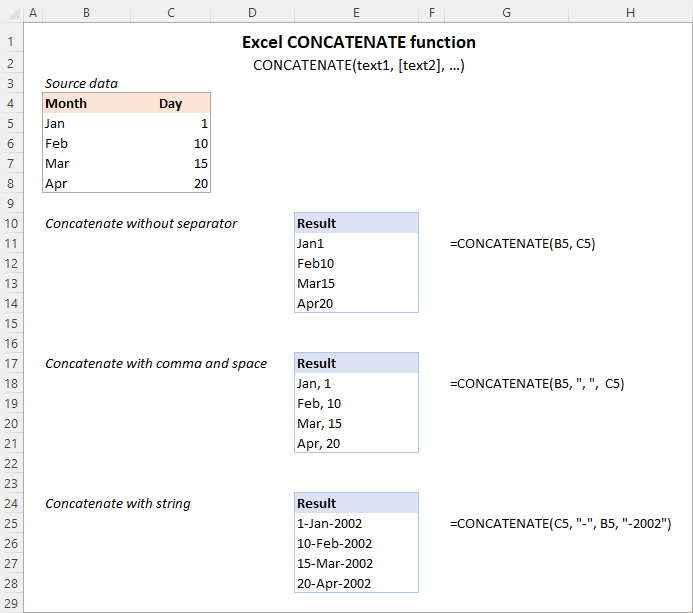
For example, to concatenate the values of B6 and C6 with a comma, the formula is:
=CONCATENATE(B6, ",", C6)
More examples are shown in the image below:
Note. In Excel 365 - Excel 2019, the CONCAT function is also available, which is a modern successor of CONCATENATE with exactly the same syntax. Although the CONCATENATE function is kept for backward compatibility, Microsoft does not give any promises that it will be supported in future versions of Excel.
Using CONCATENATE in Excel - things to remember
To ensure that your CONCATENATE formulas always deliver the correct results, remember the following simple rules:
- Excel CONCATENATE function requires at least one "text" argument to work.
- In one formula, you can concatenate up to 255 strings, a total of 8,192 characters.
- The result of the CONCATENATE function is always a text string, even when all of the source values are numbers.
- Unlike the CONCAT function, Excel CONCATENATE does not recognize arrays. Each cell reference must be listed separately. For example, you should use CONCATENATE(A1, A2, A3) and not CONCATENATE(A1:A3).
- If any of the arguments is invalid, the CONCATENATE function returns a #VALUE! error.
"&" operator to concatenate strings in Excel
In Microsoft Excel, the ampersand sign (&) is another way to concatenate cells. This method comes in very handy in many scenarios since typing an ampersand is much faster than typing the word "concatenate" :)
For example, to concatenate two cell values with a space in-between, the formula is:
=A2&" "&B2
How to concatenate in Excel - formula examples
Below you will find a few examples of using the CONCATENATE function in Excel.
Concatenate two or more cells without separator
To combine the values of two cells into one, you use the concatenation formula in its simplest form:
=CONCATENATE(A2, B2)
Or
=A2&B2
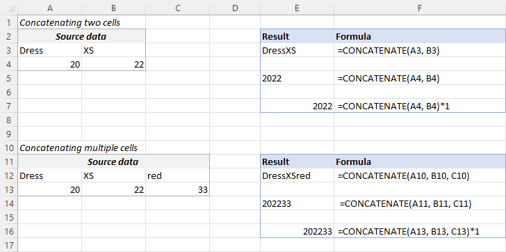
Please note that the values will be knit together without any delimiter like in the screenshot below.
To concatenate multiple cells, you need to supply each cell reference individually, even if you are combining contiguous cells. For example:
=CONCATENATE(A2, B2, C2)
Or
=A2&B2&C2
The formulas work for both text and numbers. In case of numbers, please keep in mind that the result is a text string. To convert it to number, just multiply CONCATENATE's output by 1 or add 0 to it. For instance:
=CONCATENATE(A2, B2)*1
Tip. In Excel 2019 and higher, you can use the CONCAT function to quickly concatenate multiple cells using one or more range references.
Concatenate cells with a space, comma or other delimiter
In your worksheets, you may often need to join values in a way that includes commas, spaces, various punctuation marks or other characters such as a hyphen or slash. To do this, simply put the desired character in your concatenation formula. Remember to enclose that character in quotation marks, as demonstrated in the following examples.
Concatenating two cells with a space:
=CONCATENATE(A2, " ", B2)
or
=A2 & " " & B2
Concatenating two cells with a comma:
=CONCATENATE(A2, ", ", B2)
or
=A2 & ", " & B2
Concatenating two cells with a hyphen:
=CONCATENATE(A2, "-", B2)
or
=A2 & "-" & B2
The following screenshot demonstrates how the results may look like:

Tip. In Excel 2019 and higher, you can use the TEXTJOIN function to merge strings from multiple cells with any delimiter that you specify.
Concatenating text string and cell value
There is no reason for the Excel CONCATENATE function to be limited to only joining cells' values. You can also use it to combine text strings to make the result more meaningful. For example:
=CONCATENATE(A2, " ", B2, " completed")
The above formula informs the user that a certain project is completed, as in row 2 in the screenshot below. Please notice that we add a space before the word " completed" to separate the concatenated text strings. A space (" ") is also inserted between the combined values, so that the result displays as "Project 1" rather than "Project1".
With the concatenation operator, the formula can be written this way:
=A2 & " " & B2 & " completed"
In the same manner, you can add a text string in the beginning or in the middle of your concatenation formula. For example:
=CONCATENATE("See ", A2, " ", B2)
="See " & A2 & " " & B2

Join text string and another formula
To make the result returned by some formula more understandable for your users, you can concatenate it with a text string that explains what the value actually is.
For example, you can use the following formula to return the current date in the desired format and specify what kind of date that is:
=CONCATENATE("Today is ",TEXT(TODAY(), "mmmm d, yyyy"))
="Today is " & TEXT(TODAY(), "dd-mmm-yy")

Tip. If you would like to delete the source data without affecting the resulting text strings, use the "Paste special - values only" option to convert formulas to their values.
Concatenate text strings with line breaks
Most often, you would separate the resulting text strings with punctuation marks and spaces, as shown in the previous example. In some cases, however, there may be a need to separate the values with a line break, or carriage return. A common example is merging mailing addresses from data in separate columns.
A problem is that you cannot simply type a line break in the formula like a usual character. Instead, you use the CHAR function to supply the corresponding ASCII code to the concatenation formula:
- On Windows, use CHAR(10) where 10 is the character code for Line feed.
- On Mac, use CHAR(13) where 13 is the character code for Carriage return.
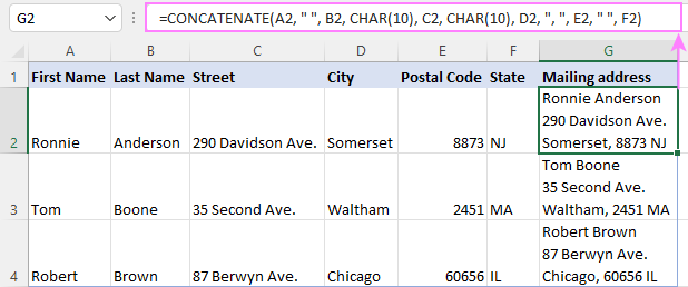
In this example, we have the address pieces in columns A through F, and we are putting them together in column G by using the concatenation operator "&". The merged values are separated with a comma (", "), space (" ") and a line break CHAR(10):
=A2 & " " & B2 & CHAR(10) & C2 & CHAR(10) & D2 & ", " & E2 & " " & F2
The CONCATENATE function would take this shape:
=CONCATENATE(A2, " ", B2, CHAR(10), C2, CHAR(10), D2, ", ", E2, " ", F2)
Either way, the result is a 3-line text string:
In the same manner, you can separate final strings with other characters such as:
- Double quotes (") - CHAR(34)
- Forward slash (/) - CHAR(47)
- Asterisk (*) - CHAR (42)
- The full list of ASCII codes is available here.
How to concatenate columns in Excel
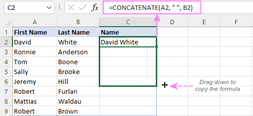
To join two or more columns, just enter your concatenation formula in the first cell, and then copy it down to other cells by dragging the fill handle (the small square that appears in the lower right hand corner of the selected cell).
For example, to combine two columns (column A and B) delimiting the values with a space, the formula in C2 copied down is:
=CONCATENATE(A2, " ", B2)
Or
= A2 & " " & B2
For more information, please see How to merge two columns in Excel without losing data.
Combine text and numbers keeping formatting
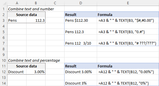
When concatenating a text string with a number, percentage or date, you may want to keep the original formatting of a numeric value or display it in a different way. This can be done by supplying the format code inside the TEXT function, which you embed in a concatenation formula.
In the beginning of this tutorial, we have already discussed a formula that concatenates text and date.
And here are a few more formula examples that combine text and number:
Number with 2 decimal places and the $ sign:
=A2 & " " & TEXT(B2, "$#,#0.00")
Number without insignificant zeros and the $ sign:
=A2 & " " & TEXT(B2, "0.#")
Fractional number:
=A2 & " " & TEXT(B2, "# ?/???")
To concatenate text and percentage, the formulas are:
Percent with two decimal places:
=A12 & " " & TEXT(B12, "0.00%")
Rounded whole percent:
=A12 & " " & TEXT(B12, "0%")
How to concatenate a range of cells in Excel
Combining values from multiple cells might take some effort because the Excel CONCATENATE function does not accept arrays.
To concatenate several cells, say A1 to A4, you need to use one of the following formulas:
=CONCATENATE(A1, A2, A3, A4)
or
=A1 & A2 & A3 & A4
When combining a fairly small group of cells, it's no big deal to type all the references. A large range would be tedious to supply, typing each individual reference manually. Below you will find 3 methods of quick range concatenation in Excel.
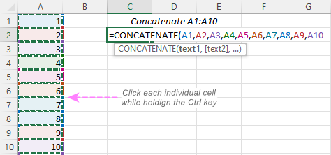
Method 1. Press CTRL to select multiple cells
To quickly select several cells, you can press and hold the Ctrl key while clicking on each cell you want to include in the formula. Here are the detailed steps:
- Select a cell where you want to enter the formula.
- Type =CONCATENATE( in that cell or in the formula bar.
- Press and hold Ctrl and click on each cell you want to concatenate.
- Release the Ctrl button, type the closing parenthesis, and press Enter.
Method 2. Use TRANSPOSE function to get all cell values
When a range consists of tens or hundreds of cells, the previous method may not be fast enough as it requires clicking on each cell. In this case, you can use the TRANSPOSE function to return an array of values, and then merge them together in one fell swoop.
- In the cell where you want the result to appear, enter the TRANSPOSE formula, for example:
=TRANSPOSE(A1:A10)
- In the formula bar, press F9 to replace the formula with calculated values. As a result, you will have an array of values to be concatenated.
- Delete the curly braces surrounding the array.

- Type =CONCATENATE( before the first value, then type the closing parenthesis after the last value, and press Enter.

Note. The result of this formula is static as it concatenates the values, not cell references. If the source data changes, you will have to repeat the process.
Method 3. Use the CONCAT function
In Excel 365 and Excel 2021, this simple formula will concatenate a range of cells in a blink:
=CONCAT(A1:A10)
Method 4. Use the Merge Cells add-in
A quick and formula-free way to concatenate any range in Excel is to use the Merge Cells add-in with the "Merge all areas in selection" option turned off, as demonstrated in Combining values of several cells into one cell.
Excel "&" operator vs. CONCATENATE function
Many users wonder which is a more efficient way to join strings in Excel - CONCATENATE function or "&" operator.
The only real difference is the 255 strings limit of the CONCATENATE function and no such limitation when using the ampersand. Other than that, there is no difference between these two methods, nor is there any speed difference between the CONCATENATE and "&" formulas.
And since 255 is a really big number and you will hardly ever need to combine that many strings in real work, the difference boils down to comfort and ease of use. Some users find CONCATENATE formulas easier to read, I personally prefer using the "&" method. So, simply stick with the technique you feel more comfortable with.
Opposite of CONCATENATE in Excel (splitting cells)
The opposite of concatenate in Excel is splitting the contents of one cell into multiple cells. This can be done in a few different ways:
- Text to Columns feature
- Flash Fill option in Excel 2013 and higher
- TEXTSPLIT function in Excel 365
- Custom formulas to split cells (MID, RIGHT, LEFT, etc.)
You can also find useful information in this article: How to unmerge cells in Excel.
Concatenate in Excel with Merge Cells add-in
With the Merge Cells add-in included in Ultimate Suite for Excel, you can efficiently do both:
- Merge several cells into one without losing data.
- Concatenate the values of several cells into a single cell and separate them with any delimiter of your choosing.
The Merge Cells tool works with all Excel versions from 2016 to 365 and can combine all data types including text strings, numbers, dates and special symbols. Its two key advantages are simplicity and speed - any concatenation is done in a couple of clicks.
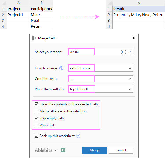
Combine values of several cells into one cell
To combine the contents of several cells, you select the range to concatenate and configure the following settings:
- Under What to merge, select Cells into one.
- Under Combine with, type the delimiter (a comma and a space in our case).
- Choose where you want to place the result.
- Most importantly, uncheck the Merge all areas in the selection box. It is this option that controls whether the cells are merged or their values are concatenated.
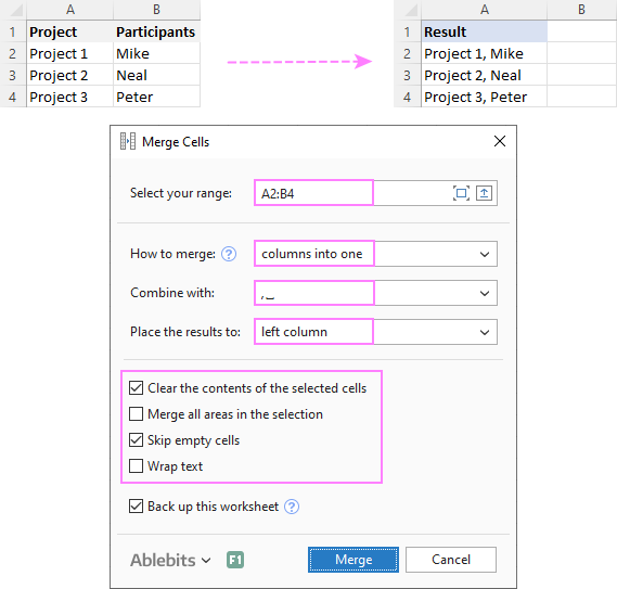
Combine columns row-by-row
To concatenate two or more columns, you configure the Merge Cells' settings in a similar way but choose to merge columns into one and place the results in the left column.
Join rows column-by-column
To combine data in each individual row, column-by-column, you choose:
- Merge rows into one.
- Use a line break for the delimiter.
- Place the results in the top row.
The result may look similar to this:
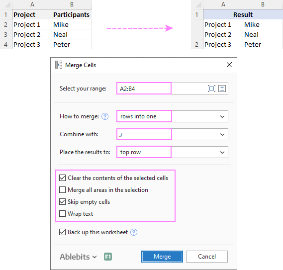
To check how the Merge Cells add-in will cope with your data sets, you are welcome to download a fully functional trial version of our Ultimate Suite for Excel below.
That's how to concatenate in Excel. I thank you for reading and hope to see you on our blog next week!
Available downloads
Concatenation formula examples (.xlsx file)
Ultimate Suite 14-day trial version (.exe file)
 by
by
447 comments
I'm trying to concatenate columns with following data to Cells
A1 A2 A3
B2 B3
C2 C3
result should be A1A2A3, A1B2B3, A1C2C3
Hello!
Please check out this article to learn how to concatenate text strings.
Try formula =CONCATENATE(A1,A2,A3,",",CONCATENATE(A1,B2,B3),",",CONCATENATE(A1,C2,C3)) this should work
Can I use concatenate to to form a reference to a defined name?
I have defined names that reference cells containing physical part subtotals in sheet WIP for each part and location combination.
PARTALOC1
PARTALOC2
PARTBLOC1
PARTBLOC2
In sheet data I have rows with PARTx in one column and LOCx in another column. Each time I run a report the data sheet may contain a different set of combinations and appear in different orders.
I can set a cell to the right of my data that will not be overwritten to concatenate and form the defined name, I can even get as for as "=partaloc1" to appear in the cell, but how do I get it to reference the name partaloc1? From what I have found about indirect it deals only with cell references, sheet names etc, but not names.
Hello!
If I understood the problem correctly, you can use the INDIRECT function.
=INDIRECT(E1)
Cell E1 contains the name as text.
In the cell you will get a link to the name.
Is there a formula for example This information together ?
For example:
Column 1- Neil
Column 2- 30295699
The result I require is NE5699 in Column 3
Not sure if this is even possible
Hi Keelan,
Assuming Neil is in A2, and 30295699 is in B2, enter one of the below formulas in C2:
=UPPER(LEFT(A2,2))&(RIGHT(B2,4))
Or
=CONCATENATE(UPPER(LEFT(A2,2)), (RIGHT(B2,4)))
How does the formula look like when I want to concatenate, say for example :JOHN FITZGERALD KENNEDY
and I want the result as "JOHN F KENNEDY" only?
Hi!
Use the LEFT function
=CONCATENATE(A2," ",LEFT(B2,1)," ",C2)
or
=TEXTJOIN(" ",TRUE,A2,LEFT(B2,1),C2)
Hope this is what you need.
I am trying to make a list where name is
John Doe email will follow jdoe@school. org
any ideas? I was able to create the password jd123456
using the formula ==CONCATENATE(LEFT(C13,2),"123456") but I ma not able to find the format
Try the following formula:
=(LOWER(CONCATENATE(LEFT(F8),(G8),"@school.org")))
F8 is First Name, G8 is Last Name.
Changed to Lower Case.
Hi,
I would like to create a table with the day sequence of a month, as ...
01/02/2021
02/02/2021
03/02/2021
but it will be a concat result of ="01/"&G$2&"/2021" for the first line, for example, where G$2 will have the number of the month I want, in this case, fev 02.
The problem is that I need the result of the concat in data format, which is not happening.
I hope it sufficiently clear to understand.
Thanks in advance.
Hello!
Enter a date in the cell. After that, you can copy this data down along the column. You will receive a sequence of days.
Or use the formula
=DATEVALUE("1/"&G2&"/2021")
I hope it’ll be helpful.
Hello : 0001 code when i use for concatination formula its shows only as 1, How to show as 0001
Hello!
Use TEXT function:
TEXT(A1)
Hope this is what you need.
The example here says to click each cell for Concatenating the cells. However, I have around 6000 records in individual cells that I need to concatenate with a semicolon. May I know the command for the same.
Example:
Car 1
Car 2
.
.
Car 5999
Car 6000
Output: Car1; Car 2; . . . Car 5999; Car 6000
Thanks in advance.
Hi!
Please have a look at this article: TEXTJOIN function in Excel to merge text from multiple cells.
I want to compare the names in two sheets,
Sheet 1: Cook Ph.D. James L.
Sheet 2: "Cook" in Last Name column , and "James" in First Name Column
I need to know the names in both sheet is same person as I don't have any unique identifiers common in both the Excel sheets.
Now instead of Ph.D it could be anything else like ABC or additional wild characters liek _ or / or -
Is there a way here?
Hello,
could someone help me to transform with a formula the first table to the second one?
ID function
L1 John
N3 Mary ID Function
D2 John L1 John, James,
L5 James N3 Mary, James
D4 John ˃ D2 John, James, Mary
N3 James L5 James
L1 James D4 John
D2 James L4 Mary
L4 Mary
D2 Mary
Thankyou
OMG, after trying for an hour to get CONCATENATE to work, I realized that you need to use a semicolon instead of a comma to separate the arguments!
It seems that all guides on this function are wrong in that regard.
Hello!
Our examples use the US regional settings. A comma is used as a separator. You are using a European settings that uses a semicolon. These regional settings are set in the Windows control panel.
Hello,
I am having trouble creating the correct CONC formula for this information. Could you please advise?
Cell Cell Data
B2 C
B3 01
B4 Data Validation- List (only want to include the first character)
B5 Data Validation-List (only want to include the first character)
B6 Data Validation- List (only want to include the first 2 characters)
B7 234
B8 Data Validation-List (only want to include the first character)
B9 21
B11 Formula that will combine cells B2-B9 in order
Thanks,
Daniela
Hello!
I am assuming CONC is CONCATENATE.
Try the following formula:
=CONCATENATE(B2,B3,LEFT(B4,1),LEFT(B5,1),LEFT(B6,1),B7,LEFT(B8,1),B9)
I hope this will help
Hi,
If am using Concatenation then what will be the formula when I have go drag the same for number of rows and columns at time???
Ex. If I have to drag same formula for rows I'll add $ for column number and wise versa.
Them what about doing both draging at a time???
Thanks
Hello!
Please check out the following article on our blog, it’ll be sure to help you with your task: How to copy formula in Excel with or without changing references
I hope it’ll be helpful.
Thanks very much for tutorials, I like to know if there is a way to concatenate my data which is in single column having following format:
Addition Cost 30-
SEP-2005 00:00:00
Addition Cost 31-
OCT-2005 00:00:00
Addition Cost 31-
MAR-2006 00:00:00
Addition Cost 28-
FEB-2007 00:00:00
Reclass Cost 31-MAR-
2007 00:00:00
Addition Cost 31-
MAR-2007 00:00:00
As per format provided all i want is to concatenate every consecutive line before a blank row occurs in the following desired format:
Addition Cost 30-SEP-2005 00:00:00
Addition Cost 31-OCT-2005 00:00:00
Addition Cost 31-MAR-2006 00:00:00
Addition Cost 28-FEB-2007 00:00:00
Reclass Cost 31-MAR-2007 00:00:00
Addition Cost 31-MAR-2007 00:00:00
I have thousands of rows in my data, is there any way that concatenate function can be nested with IF function to concatenate rows between every blank rows.
Thanks in advance if someone can help me please!
Hi, I was wondering if there's a way to concatenate all permutations within 3 columns and let's say 20 rows. So the obvious would be a2+b2+c2, a3+b3+c3 etc... but I also want a2+b3+c2, and a2 +b3 +c4, and a2+b2+c7 etc etc etc. all the way to a20+b20+c20 in all permutations in between. Is there a formula for this?
Is there a way to concatenate cells across multiple rows IF you there is a repeated value in another column? Here's my scenario.
THIS IS MY RAW DATA SET:
COLUMN A COLUMN B
ABC PRODUCT 1
ABC PRODUCT 2
ABC PRODUCT 3
ABC PRODUCT 4
XYZ PRODUCT 1
XYZ PRODUCT 2
XYZ PRODUCT 3
THIS IS THE RESULT I WANT:
COLUMN A COLUMN B
ABC PRODUCT 1; PRODUCT 2; PRODUCT 3; PRODUCT 4
XYZ PRODUCT 1; PRODUCT 2; PRODUCT 3
Thank you in advance for your help.
can you help simple formula like number 12345678879093879, to be =12+34+56+78+87+90+93+87+9 (546) and add "+" every 2 number after but later result sum that all number?
Hello!
You can only convert text to a formula using a VBA macro. You can split these numbers by cells and then find their sum.
Is this how I can replace text in Column B with text in Column A?
For example, Column A has R210#P and Column B has INSERT:IMG_PREMIUM_R210#K_ARTISTLASTNAME.
I want to replace the R210#K in Column B with the R210#P in Column A.
Hello!
If the value R210#P is written in cell B1, then it cannot be changed using an Excel formula. This can only be done with the VBA macro. A cell can contain either a value or a formula. The formula cannot change the value of another cell.
=CONCATENATE(MONTH(Table_Query_form_DMSlink[[#this Row],[ordre Date]]),"/Year(B15)) please explan this
Hello!
Your task is not completely clear to me. It is very difficult to understand a formula that contains unique references to your workbook worksheets. Hence, I cannot check its work, sorry. Please specify what you were trying to find, what formula you used and what problem or error occurred.
How do I concatenate a name and phone number (different cells)
Sheet1!I1= Jane Dow
Sheet1!J1 = (000) 000-0000
Into one cell to read
Jane Doe (000) 000-000
Hello!
Pay attention to the following paragraph of the article above Concatenate cells with space
i need to know after 5 digit how put -ve sign 921023E550 ( example 92102-3E550 )
please inform us the formula
Hello!
If I understand your task correctly, the following formula should work for you:
=LEFT(F1,5)&"-"&RIGHT(F1,LEN(F1)-5)
Hope this is what you need.
I am trying to concatenate two separate data sets where all the data in A get's repeated for each cell in B. Is there a way to concatenate this without manually changing the $ for each cell in the concatenate function?
example:
Origin Zone Destination Zones
BTD-TGD 32218
NOD-BBK 90670
NOD-BBK-BTD 90749
The result I am looking for is:
BTD-TGD_32218
NOD-BBK_32218
NOD-BBK-BTD_32218
BTD-TGD_90670
NOD-BBK_90670
NOD-BBK-BTD_90670
And so on. Currently the only way I know to do this is =CONCATENATE(A1,"_"b$2) and then change to (...b$3) when all of the data for b2 has been completed.
Hello!
We have a tool that can solve your task in a couple of clicks: Ablebits Tools- Create Cards.
If your data is written in 3 columns -
aaa bbb ccc
123 123 123
456 456 456
789 789 789
and set Number of columns to 1 and "Add header"б
then we get the result -
aaa 123
bbb 123
ccc 123
aaa 456
bbb 456
ccc 456
aaa 789
bbb 789
ccc 789
This tool is available as a part of our Ultimate Suite for Excel that you can install in a trial mode and use for free: https://www.ablebits.com/files/get.php?addin=xl-suite&f=free-trial
If you have any (other) questions, don't hesitate to ask.
I am building a list for a team to use that has unique hyperlinks in each row of data. I have attempted to use concatenate to add the active link to a sentence of text. Simply using concatenate, the link does not stay active. Using & the entire text becomes an active link. Is there another operator I should be adding?
Hello!
I’m sorry but your task is not entirely clear to me. For me to be able to help you better, please describe your task in more detail. Please specify what you were trying to find, what formula you used and what problem or error occurred. Give an example of the source data and the expected result.
It’ll help me understand it better and find a solution for you. Thank you.
Need help...
What if i want to concatenate in excel then i also want to add a open expression
Column A = 2+1
Column B = Roses
Column C = Concatenate(A&" "&B)
Result currently as 2+1 Roses but what i need to know is how can i covert it automatically to 3 Roses
Thanks in advance
Hello!
Cell A1 now contains the text "2 + 1". If you change it to the formula = 2 + 1, then you will get the desired result.
a1
a2 a20
how we drag a20 by using concatenate pls help
Hi,
How to auto concatenate a RANGE of Cells before space:
List 1 List 2 Concated list
AA MM MM
CC PP PP QQ
CC QQ
DD TT TT MM NN
DD MM
DD NN
thank
Hello Svetlana,
"Excellent" also can not describe the good work you have done and it's being explained in such a easy manner even a layman will become an expert in Excel.
Great work keep it up.
God bless you.
Cheers,
Yogesh
HI I am trying to work out the following formatting and was hoping you could help.
If I have a range of 90% to 100% in a cell K5 in the next cell K6 I would like it to say excellent
but if in that cell I have a range of 80% to 89% I would like it to say very good.
basically its a if this then that... but not with colors with specific text.
Hello Alexander,
I have a number of cells to concatenate in order to generate an unique identifier for each line item.
The cells contain, for example - A2: 200729, B2: SNK, C2: 34543
My formula reads: =concatenate(right(A2,3),"-",B2,"-",left(C2,2)) producing 729-SNK-34
In cell A2, I would like to use the second digit "0" at the beginning of the unique identifier, so need to skip the first digit in cell A2 and use the second, while the rest of the formula stays the same....so the result should then read 0729-SNK-34. Is that possible please...and thank you!
Hello!
If I understand your task correctly, the following formula should work for you:
=CONCATENATE(REPLACE(A2,1,2,""),"-",B2,"-",LEFT(C2,2))
I hope this will help
Is there a way to exclude two specific characters whenever they appear in the cells that you are combining? Either using CONCATENATE or any other function. For example:
A2 thru A5 all have the same data: AA .
B2 thru B5 have: T-14 T-14+ T-14= T-14++= in which the hyphen, plus sign, and equals sign are not actually mathematical, but rather are part of the "model number" (no idea why). That is, they are just textual, not math.
C2 thru C5 have the data: 22 33 44 55.
I need to place the letter X then Cell A then Cell B then Cell C together, eliminating any plus signs or equals (remember, they are not mathematical). The hyphens can stay.
I tried this: =("X"&A5&(SUBSTITUTE(B5,"+",""))&C5)
It of course doesn't eliminate the "=" symbol. I get the result I want for Rows 2 and 3, for example XAAT-1422, XAAT-1433. And not the result that I want for Rows 4 and 5, which return these results: XAAT-14=44, XAAT-14=55.
And vice versa if I use =("X"&A5&(SUBSTITUTE(B5,"=",""))&C5)
I get my desired result for Rows 2 and 4 (XAAT-1422, XAAT-1444) but not for rows 3 and 5, which return XAAT-14+33 and XAAT-14++55.
So I want to be able to eliminate all + symbols and = symbols. I know this scenario is odd to use these symbols, and not mathematically, but the manufacturer uses them in model naming. Thank you for any help! I had started with a concatenate function but couldn't get it to work for me either.
Clarification as the spacing above makes it hard to read what I intended:
B2 thru B5 have:
T-14
T-14+
T-14=
T-14++=
in which the hyphen, plus sign, and equals sign are not actually mathematical, but rather are part of the "model number" ..
Hello Jillian!
If I understand your task correctly, the following formula should work for you:
="X"&A2&SUBSTITUTE(SUBSTITUTE(B2,"=",""),"+","")&C2
or
=CONCATENATE("X",A3,SUBSTITUTE(SUBSTITUTE(B3,"=",""),"+",""),C3)
I hope it’ll be helpful.
Hello!
I have a sales record covering 3 years and i want to report on the highest sales made per year. Can i nest the (=Max) function into a (=Concat) one?
So that it reads "Gross sales for 2018 were highest at $35000"
Hello!
Of course you can use something like this
=CONCAT("Gross sales for 2018 were highest at $",MAX(C1:C18))
Function arguments can be text, numbers, cell references, other Excel functions
How to insert a character in the middle of string/number?
eg: 12345 -> 123-45
Hello!
If I understand your task correctly, the following formula should work for you:
=CONCATENATE(LEFT(B12,ROUND(LEN(B12)/2,0)),"-", RIGHT(B12,LEN(B12)-ROUND(LEN(B12)/2,0)))
Hope this is what you need.
I would like to create a password generator, using a list of words. Then be able to grab 4 random words.
I can create a number with RANDBETWEEN, but how do I convert that to a cell to CONCATENATE?
I think I solved my own question, this may not be the most elegant, but it worked.
I have a list of words, numbers, and symbols in column I. 1 to 8000
I want 4 random words combined together from the list of 8000
Created four cells with =RANDBETWEEN(1,8000) let us assume the 4 cells created are L1, M1,N1, and O1
in cell P1 I have =CONCATENATE("I",L1)
in cell Q1 I have =CONCATENATE("I",M1)
in cell R1 I have =CONCATENATE("I",N1)
and in cell S1 I have =CONCATENATE("I",O1)
Then in T1 I have
=CONCATENATE((INDIRECT(P1)),"-",(INDIRECT(P1)),"-",(INDIRECT(Q1),"-",(INDIRECT(S1)))
This returns word-made-up-password (of course the words in those cell in column I are different.
Is there a better way?
Correction:
=CONCATENATE((INDIRECT(P1)),"-",(INDIRECT(Q1)),"-",(INDIRECT(R1),"-",(INDIRECT(S1)))
Hello Tom!
If RANDBETWEEN selects numbers, for example, from 1 to 10, then each number can correspond to a word using the CHOOSE function. If you describe in more detail your task, initial data and the desired result, I can give more detailed advice.
I want to concatenate on my userform says: (Balance: and 10,000)Note 10,000 is a value on a textbox which can be different by selecting another information.
Hello!
I hope you have studied the recommendations in the above tutorial. If I got you right, the formula below will help you with your task:
=CONCATENATE("Balance: ",A1)
I hope this will help
I am trying to get the cell to read:
Assessed: 18%
Current Formula
="Assessed: "&('C&BE'!E29/'C&BE'!E24)
I want the text 'Assessed: ' and then I want to have the number 18% which comes from a different tab where 2 items are divided. This is what I get 'Assessed: 0.181818181818182' All I want to do is get this number to be a percentage but I can't seem to convert it to percentage. Using the 'Number Format' or 'Display Percentage' items don't convert it. Format Cell doesn't work. It's almost like the '&' function seems to negate these properties. [I have Mac 2011 version 14.7.7 (170905)
I'm looking for the exact same function. Have you found a solution?
Hello!
The formula below will do the trick for you:
=E24&" "&TEXT(E29,"###%")
or
=CONCATENATE(E24," ",TEXT(E29,"###%"))
Hope this is what you need.
Hello..
In excel all the data is in Cell A1 coloumn and rows 1,2,3 so on. So i want to combine the name in Cell B1 coloumn.. So i am combine two rows using this formula =A1&A2 but i am facing problm that all the name are not belong in 2 rows they are separate in 3 rows or 4 rows.
Example -
Buff Milano
Dk. Cog
Buff Milano
Red
Buff Milano
Grade B
Black
Buff Milano
Grade B
Black
In this way i have a huge coloumn can any one solve my problem.. Is there any formula
Note :
I wan to find out this in Coloumn B -
Buff Milano Dk. Cog
Buff Milano Red
Buff Milano Grade B Black
Is there a way to concatenate an array (obtained as a result of a formula in a cell)?
Hello!
The CONCATENATE function and the & operator cannot combine a range of cells. Therefore, it is impossible to write a formula. You can use VBA or our ready-made solution.
I'd recommend you to have a look at our Ablebits Data - Merge Cells.
This tool is available as a part of our Ultimate Suite for Excel that you can install in a trial mode and use for 30 days for free: https://www.ablebits.com/files/get.php?addin=xl-suite&f=free-trial
I want to know how to store alternate values in one cell. I am doing some soccer related collation using microsoft excel. For instance cell A1 is barcelona and cell B1 is juventus. I want cell C1 to represent barcelona OR juventus, I don't want cell C1 to represent barcelona AND juventus
Hello!
I recommend that you study the article on our blog about IF function with several conditions.
Before reading this article I concatenated cells by using the method of = and the cells I wanted, separated by spaces for the most part. This is my formula:
= ( "Requisition" & " " & A39 &" : " & B39 & "- "& C39 & " - " & D39 & " " & E39)
One of my cells was in currency (it was Cell E39). How can I make the information (the currency) hold its format when transferred to the next cell?
F39 holds all the information input from A39 to E39. But when the information in E39 is transferred to F39, instead of seeing $210,000.00 I see 210000.
Hi Is there any way to concat General non-text fields and output the result as a numeric? eg:
Order Version Output as a number
1234 1 12341
1234 2 12342
Thanks
Hello Gary!
If I understand your task correctly, please try the following formula:
=VALUE(A1&B1)
I hope this will help, otherwise please do not hesitate to contact me anytime.
How can I concatenate values from two cells in to one cell, but skip few letters from one of the cell. For example.
Cell A1 has - Mr Joe
Cell B1 has - Smith
Cell C1 should print "Joe Smith" skipping "Mr" from Cell A1 values.
Hello Matt!
The number of characters to skip is unknown. It can be from 0 to 4. Therefore, it is impossible to write a formula. You can use VBA or our ready-made solution.
I'd recommend you to have a look at our Ablebits Tools - Split Names.
This tool is available as a part of our Ultimate Suite for Excel that you can install in a trial mode and use for 30 days for free: https://www.ablebits.com/files/get.php?addin=xl-suite&f=free-trial
How can I concatenate a data from regional data to a new sheet
Hello Jossy!
For me to be able to help you better, please describe your task in more detail. It’ll help me understand it better and find a solution for you. Thank you.
I want to add concatenate formula but to remove some text from the existing values..
How can i do that
Hello!
For me to be able to help you better, please describe your task in more detail. It’ll help me understand it better and find a solution for you. Thank you.
I want sum of marks on sheet1 based on students count in Sheet marks and student count is located in sheet2
I use formula count if to count students in a2 cell in sheet2
In case i have 27 students
A2=27
Marks starts from row number 10
I want sum of E coloum in sheet1
E10 to value of A2+9=27
My all sheets have different number of students
And all sheets have count of students in A2 cell in perticular sheet.
Help me
If I have two cells, each with a formula to display length of service (years, months and days), is there a way for me to calculate the total of the years, months and days for each cell into one?
Thanks!
Any way to retain individual cell formatting (i.e., bold for the first element) in the concatenated cell?
Very helpfull thanks
Hi,
Is there a way where I can concatenate three different cells by keeping one cell value as constant output
A Output
10 20 A;10;20
15 21 A;15;21
17 22 A;17:22
Please suggest best formula to create above output. Thanks in Advance!!
Suppose I have a file with columns A1:C3.
Column A (A1:A3)= Apple, Banana, Carrot (each word in a separate row)
Column B (B1:B3)= Red, Yellow, Orange (each word in a separate row)
Column C (C1:C3)= Y, N, Y (each word in a separate row)
I'd like to concatenate the words in column A into cell D1 contingent upon the value in the C column is "Y". For example I'd like the formula in D1 to return "Apple, Carrot" because Both A1 (Apple) and A3 (Carrot) have C1 and C3 with a "Y" string. Is there a way to concatenate with an IF statement argument in a separate column from what is being combined? Thanks in advance for your help!
All the best,
Whitney
While you could do something like
=CONCATENATE(IF(A$3="Y";A1;"");" ";IF(B$3="Y";B1;"");" ";IF(C$3="Y";C1;"")),
this would only work for a fixed range and for every column you would have to change the IF. What I would suggest is making an equivalent amount of columns to those you wish to concatenate, and populate them with =IF(A$3="Y";A1;""), and then combine those with concatenate.
I would use an extra column, a working scratchpad column, hide it if you don't want it seen. E column where E1 is "IF(C1="Y", A1, "")". In other words, if C is Y, then copy A, otherwise make the cell blank. Then where you want the concatenated string, just "E1&E2&E3" (though I would think A4 is a more logical destination, this is essentially SUMIF but with text). The commas are harder, to not have one on the last. I would do "IF(C1="Y", A1&", ", "")" so all entries end in a comma, then in E4 put the concatenation, then where you WANT the concatenation you put "LEFT(E4, LEN(E4)-2)". That way E4 is your target string but ending with an extra comma and space, so this would remove them.
Is it possible to convert a concatenated formula to an actual formula?
For example, I have 4 columns with the following:
='TM Receipts',!,P,16
I concatenate those 4 columns to get "='TM Receipts'!P16"
This is still a text string of course and I want to convert it a formula to give me the actual value of cell P16 on the TM Receipts worksheet.
Is there a way to do this?
In other words, you want to then retrieve the contents of this P16... You want the command "INDIRECT". The argument it takes is a cell address you want to get, so in your example "INDIRECT("'TM Receipts'!P16"), useful for when you have to use a formula to construct an address. I use formulas like "INDIRECT("A"&(B1*8)+1)" all the time (where A is filled with identical groups of information taking 8 rows each, B is sequential numbers starting from 0, and I'm looking for the first row of each group. On line 0 this become A1, I get A1. On line 1 it's A9, etc). Be warned, formulas with INDIRECT don't update like other formulas do, so if you insert a row above P so that your data moves down one, INDIRECT doesn't care, it'll still get whatever is now in P16.
I am not having any luck with this but I might be applying it incorrectly. I am trying to return the results in row 25 and a variable column. So in, say, D1 I would enter 'B' and then I'd get the value of B25. Unfortunately, =INDIRECT(D1 & "25") is returning 0 though. I hope that makes sense as I've been working on this for way too long and my brain is fried.
after you have entered CONCATENATE formula, press.. F2 > F9 > Enter