In this article, you will learn various ways to concatenate text strings, numbers and dates in Excel using the CONCATENATE function and "&" operator. We will also discuss formulas to combine individual cells, columns and ranges.
In your Excel workbooks, the data is not always structured according to your needs. Often you may want to split the content of one cell into individual cells or do the opposite - combine data from two or more columns into a single column. Common examples are joining names and address parts, combining text with a formula-driven value, displaying dates and times in the desired format, to name a few.
In this tutorial, we are going to explore various techniques of Excel string concatenation, so you can choose the method best suited for your worksheets.
What is "concatenate" in Excel?
In essence, there are two ways to combine data in Excel spreadsheets:
- Merging cells
- Concatenating cells' values
When you merge cells, you "physically" join two or more cells into a single cell. As a result, you have one larger cell that is displayed across multiple rows and/or columns.
When you concatenate cells in Excel, you combine only the contents of those cells. In other words, concatenation in Excel is the process of joining two or more values together. This method is often used to combine a few pieces of text that reside in different cells (technically, these are called text strings or simply strings) or insert a formula-calculated value in the middle of some text.
The following screenshot demonstrates the difference between these two methods:

Merging cells in Excel is the subject of a separate article, and in this tutorial, we'll discuss the two main ways to concatenate strings in Excel - by using the CONCATENATE function and the concatenation operator (&).
Excel CONCATENATE function
The CONCATENATE function in Excel is used to join different pieces of text together or combine values from several cells into one cell.
The syntax of Excel CONCATENATE is as follows:
Where text is a text string, cell reference or formula-driven value.
The CONCATENATE function is supported in all versions of Excel 365 - 2007.
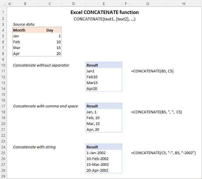
For example, to concatenate the values of B6 and C6 with a comma, the formula is:
=CONCATENATE(B6, ",", C6)
More examples are shown in the image below:
Note. In Excel 365 - Excel 2019, the CONCAT function is also available, which is a modern successor of CONCATENATE with exactly the same syntax. Although the CONCATENATE function is kept for backward compatibility, Microsoft does not give any promises that it will be supported in future versions of Excel.
Using CONCATENATE in Excel - things to remember
To ensure that your CONCATENATE formulas always deliver the correct results, remember the following simple rules:
- Excel CONCATENATE function requires at least one "text" argument to work.
- In one formula, you can concatenate up to 255 strings, a total of 8,192 characters.
- The result of the CONCATENATE function is always a text string, even when all of the source values are numbers.
- Unlike the CONCAT function, Excel CONCATENATE does not recognize arrays. Each cell reference must be listed separately. For example, you should use CONCATENATE(A1, A2, A3) and not CONCATENATE(A1:A3).
- If any of the arguments is invalid, the CONCATENATE function returns a #VALUE! error.
"&" operator to concatenate strings in Excel
In Microsoft Excel, the ampersand sign (&) is another way to concatenate cells. This method comes in very handy in many scenarios since typing an ampersand is much faster than typing the word "concatenate" :)
For example, to concatenate two cell values with a space in-between, the formula is:
=A2&" "&B2
How to concatenate in Excel - formula examples
Below you will find a few examples of using the CONCATENATE function in Excel.
Concatenate two or more cells without separator
To combine the values of two cells into one, you use the concatenation formula in its simplest form:
=CONCATENATE(A2, B2)
Or
=A2&B2
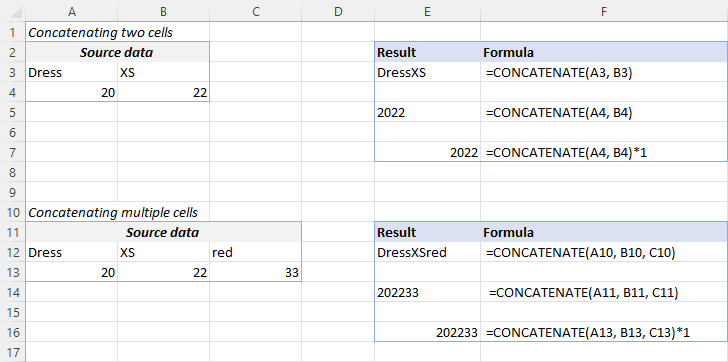
Please note that the values will be knit together without any delimiter like in the screenshot below.
To concatenate multiple cells, you need to supply each cell reference individually, even if you are combining contiguous cells. For example:
=CONCATENATE(A2, B2, C2)
Or
=A2&B2&C2
The formulas work for both text and numbers. In case of numbers, please keep in mind that the result is a text string. To convert it to number, just multiply CONCATENATE's output by 1 or add 0 to it. For instance:
=CONCATENATE(A2, B2)*1
Tip. In Excel 2019 and higher, you can use the CONCAT function to quickly concatenate multiple cells using one or more range references.
Concatenate cells with a space, comma or other delimiter
In your worksheets, you may often need to join values in a way that includes commas, spaces, various punctuation marks or other characters such as a hyphen or slash. To do this, simply put the desired character in your concatenation formula. Remember to enclose that character in quotation marks, as demonstrated in the following examples.
Concatenating two cells with a space:
=CONCATENATE(A2, " ", B2)
or
=A2 & " " & B2
Concatenating two cells with a comma:
=CONCATENATE(A2, ", ", B2)
or
=A2 & ", " & B2
Concatenating two cells with a hyphen:
=CONCATENATE(A2, "-", B2)
or
=A2 & "-" & B2
The following screenshot demonstrates how the results may look like:

Tip. In Excel 2019 and higher, you can use the TEXTJOIN function to merge strings from multiple cells with any delimiter that you specify.
Concatenating text string and cell value
There is no reason for the Excel CONCATENATE function to be limited to only joining cells' values. You can also use it to combine text strings to make the result more meaningful. For example:
=CONCATENATE(A2, " ", B2, " completed")
The above formula informs the user that a certain project is completed, as in row 2 in the screenshot below. Please notice that we add a space before the word " completed" to separate the concatenated text strings. A space (" ") is also inserted between the combined values, so that the result displays as "Project 1" rather than "Project1".
With the concatenation operator, the formula can be written this way:
=A2 & " " & B2 & " completed"
In the same manner, you can add a text string in the beginning or in the middle of your concatenation formula. For example:
=CONCATENATE("See ", A2, " ", B2)
="See " & A2 & " " & B2

Join text string and another formula
To make the result returned by some formula more understandable for your users, you can concatenate it with a text string that explains what the value actually is.
For example, you can use the following formula to return the current date in the desired format and specify what kind of date that is:
=CONCATENATE("Today is ",TEXT(TODAY(), "mmmm d, yyyy"))
="Today is " & TEXT(TODAY(), "dd-mmm-yy")

Tip. If you would like to delete the source data without affecting the resulting text strings, use the "Paste special - values only" option to convert formulas to their values.
Concatenate text strings with line breaks
Most often, you would separate the resulting text strings with punctuation marks and spaces, as shown in the previous example. In some cases, however, there may be a need to separate the values with a line break, or carriage return. A common example is merging mailing addresses from data in separate columns.
A problem is that you cannot simply type a line break in the formula like a usual character. Instead, you use the CHAR function to supply the corresponding ASCII code to the concatenation formula:
- On Windows, use CHAR(10) where 10 is the character code for Line feed.
- On Mac, use CHAR(13) where 13 is the character code for Carriage return.
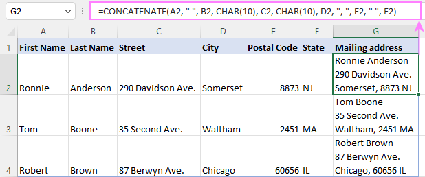
In this example, we have the address pieces in columns A through F, and we are putting them together in column G by using the concatenation operator "&". The merged values are separated with a comma (", "), space (" ") and a line break CHAR(10):
=A2 & " " & B2 & CHAR(10) & C2 & CHAR(10) & D2 & ", " & E2 & " " & F2
The CONCATENATE function would take this shape:
=CONCATENATE(A2, " ", B2, CHAR(10), C2, CHAR(10), D2, ", ", E2, " ", F2)
Either way, the result is a 3-line text string:
In the same manner, you can separate final strings with other characters such as:
- Double quotes (") - CHAR(34)
- Forward slash (/) - CHAR(47)
- Asterisk (*) - CHAR (42)
- The full list of ASCII codes is available here.
How to concatenate columns in Excel
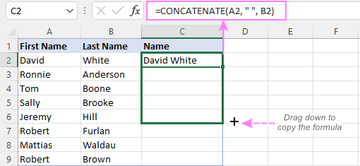
To join two or more columns, just enter your concatenation formula in the first cell, and then copy it down to other cells by dragging the fill handle (the small square that appears in the lower right hand corner of the selected cell).
For example, to combine two columns (column A and B) delimiting the values with a space, the formula in C2 copied down is:
=CONCATENATE(A2, " ", B2)
Or
= A2 & " " & B2
For more information, please see How to merge two columns in Excel without losing data.
Combine text and numbers keeping formatting
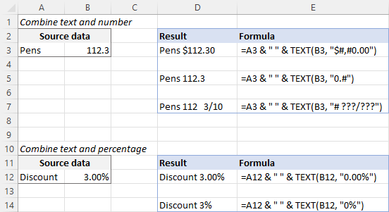
When concatenating a text string with a number, percentage or date, you may want to keep the original formatting of a numeric value or display it in a different way. This can be done by supplying the format code inside the TEXT function, which you embed in a concatenation formula.
In the beginning of this tutorial, we have already discussed a formula that concatenates text and date.
And here are a few more formula examples that combine text and number:
Number with 2 decimal places and the $ sign:
=A2 & " " & TEXT(B2, "$#,#0.00")
Number without insignificant zeros and the $ sign:
=A2 & " " & TEXT(B2, "0.#")
Fractional number:
=A2 & " " & TEXT(B2, "# ?/???")
To concatenate text and percentage, the formulas are:
Percent with two decimal places:
=A12 & " " & TEXT(B12, "0.00%")
Rounded whole percent:
=A12 & " " & TEXT(B12, "0%")
How to concatenate a range of cells in Excel
Combining values from multiple cells might take some effort because the Excel CONCATENATE function does not accept arrays.
To concatenate several cells, say A1 to A4, you need to use one of the following formulas:
=CONCATENATE(A1, A2, A3, A4)
or
=A1 & A2 & A3 & A4
When combining a fairly small group of cells, it's no big deal to type all the references. A large range would be tedious to supply, typing each individual reference manually. Below you will find 3 methods of quick range concatenation in Excel.
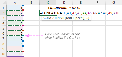
Method 1. Press CTRL to select multiple cells
To quickly select several cells, you can press and hold the Ctrl key while clicking on each cell you want to include in the formula. Here are the detailed steps:
- Select a cell where you want to enter the formula.
- Type =CONCATENATE( in that cell or in the formula bar.
- Press and hold Ctrl and click on each cell you want to concatenate.
- Release the Ctrl button, type the closing parenthesis, and press Enter.
Method 2. Use TRANSPOSE function to get all cell values
When a range consists of tens or hundreds of cells, the previous method may not be fast enough as it requires clicking on each cell. In this case, you can use the TRANSPOSE function to return an array of values, and then merge them together in one fell swoop.
- In the cell where you want the result to appear, enter the TRANSPOSE formula, for example:
=TRANSPOSE(A1:A10)
- In the formula bar, press F9 to replace the formula with calculated values. As a result, you will have an array of values to be concatenated.
- Delete the curly braces surrounding the array.

- Type =CONCATENATE( before the first value, then type the closing parenthesis after the last value, and press Enter.

Note. The result of this formula is static as it concatenates the values, not cell references. If the source data changes, you will have to repeat the process.
Method 3. Use the CONCAT function
In Excel 365 and Excel 2021, this simple formula will concatenate a range of cells in a blink:
=CONCAT(A1:A10)
Method 4. Use the Merge Cells add-in
A quick and formula-free way to concatenate any range in Excel is to use the Merge Cells add-in with the "Merge all areas in selection" option turned off, as demonstrated in Combining values of several cells into one cell.
Excel "&" operator vs. CONCATENATE function
Many users wonder which is a more efficient way to join strings in Excel - CONCATENATE function or "&" operator.
The only real difference is the 255 strings limit of the CONCATENATE function and no such limitation when using the ampersand. Other than that, there is no difference between these two methods, nor is there any speed difference between the CONCATENATE and "&" formulas.
And since 255 is a really big number and you will hardly ever need to combine that many strings in real work, the difference boils down to comfort and ease of use. Some users find CONCATENATE formulas easier to read, I personally prefer using the "&" method. So, simply stick with the technique you feel more comfortable with.
Opposite of CONCATENATE in Excel (splitting cells)
The opposite of concatenate in Excel is splitting the contents of one cell into multiple cells. This can be done in a few different ways:
- Text to Columns feature
- Flash Fill option in Excel 2013 and higher
- TEXTSPLIT function in Excel 365
- Custom formulas to split cells (MID, RIGHT, LEFT, etc.)
You can also find useful information in this article: How to unmerge cells in Excel.
Concatenate in Excel with Merge Cells add-in
With the Merge Cells add-in included in Ultimate Suite for Excel, you can efficiently do both:
- Merge several cells into one without losing data.
- Concatenate the values of several cells into a single cell and separate them with any delimiter of your choosing.
The Merge Cells tool works with all Excel versions from 2016 to 365 and can combine all data types including text strings, numbers, dates and special symbols. Its two key advantages are simplicity and speed - any concatenation is done in a couple of clicks.
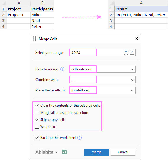
Combine values of several cells into one cell
To combine the contents of several cells, you select the range to concatenate and configure the following settings:
- Under What to merge, select Cells into one.
- Under Combine with, type the delimiter (a comma and a space in our case).
- Choose where you want to place the result.
- Most importantly, uncheck the Merge all areas in the selection box. It is this option that controls whether the cells are merged or their values are concatenated.
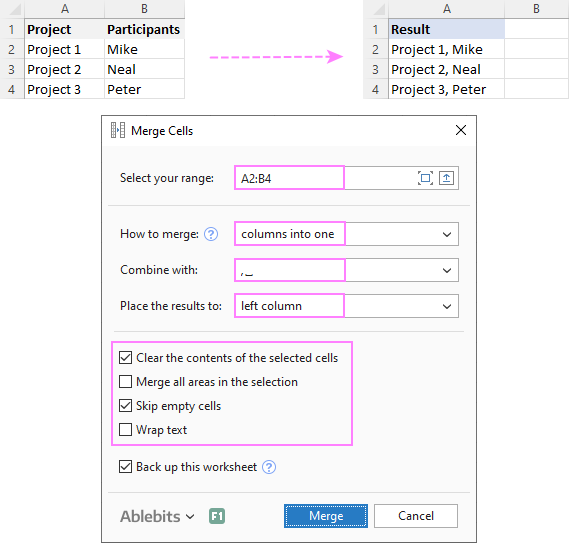
Combine columns row-by-row
To concatenate two or more columns, you configure the Merge Cells' settings in a similar way but choose to merge columns into one and place the results in the left column.
Join rows column-by-column
To combine data in each individual row, column-by-column, you choose:
- Merge rows into one.
- Use a line break for the delimiter.
- Place the results in the top row.
The result may look similar to this:
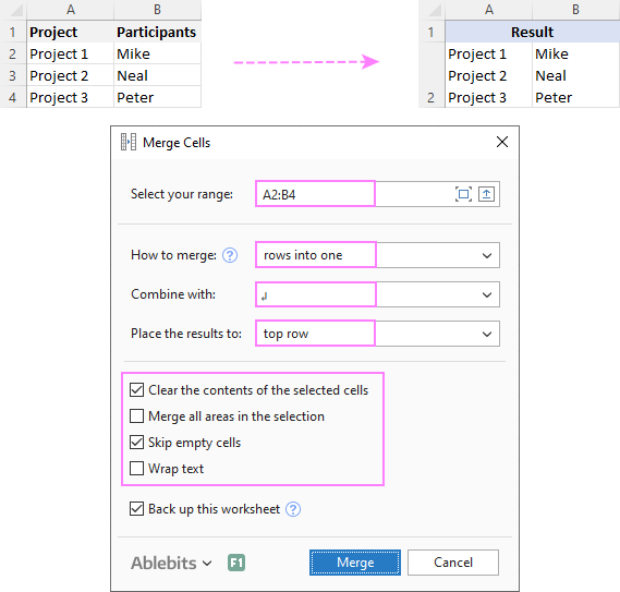
To check how the Merge Cells add-in will cope with your data sets, you are welcome to download a fully functional trial version of our Ultimate Suite for Excel below.
That's how to concatenate in Excel. I thank you for reading and hope to see you on our blog next week!
Available downloads
Concatenation formula examples (.xlsx file)
Ultimate Suite 14-day trial version (.exe file)
 by
by
447 comments
I have a doubt with concatenate with time, fr example i have abc123456 in A1 and 4.00 PM in B1 so if i use the formula the time changes to 0.666667. can you help me with that.
Use CONCATENATE(A1;" ";TEXT(B1;"h.mm AM/PM")
Hi there, I'm trying to Concatenate two cells but my formula cell just displays the formula not the answer. Cell F23 has 'KM 11510', Cell G23 has 'Sheet Music and Document Holder'. I used the function library and the Function Arguments show the Formula Result = 'KM 11510 Sheet Music and Document Holder', which is what I want. But when I press OK, the field shows =CONCATENATE(F23," ",G23). I have checked that Calculation Options are on Automatic. I've tried switching it to manual and back, I've tried saving and re-opening. any suggestions? Thanks very much.
hi
im having an issue using a formula on a multiple cells
like i want to get a text when i put something in a multiple cells
thankyou sir
hi,
i want to add rows having same names for ex
columnA columnB
A 1
A 2
A 3
B 1
B 2
C 1222
C 2121
Which formula is usefull for this??
We maintain medical equipments purchase, sales, stock sl.no. wise. Example of sl. No.is ASHD-7891, ASDG-2367 etc. How advance excel recognize these sl nos
How do I take a column of numbers and put it in one cell separated by commas.
(123,234,345,456,678) I want this result
Hi,
Please share how can we concatenate list of cells values with comma, like A,B,C
Table
P2-G021
P2-6704
P2-3045
P2-I172
P2-6056
P2-I046
P2-1582
Thanks
Harish
How can i print the report as given below
Source
RAJA 500 3
RAJA 300 4
SHYAM 200 5
SHYAM 300 4
SHYAM 100 3
VENU 200 4
RESULT
RAJA 500/3, 300/4
SHYAM 200/5, 300/4, 100/3
VENU 200/4
Please reply
Hi,
Am trying to create a production planning sheet where I have to provide data with comma separators for the values for convenient reading.
When I use concatenate function I cannot get the commas in the middle.
When I use the function it return 100000 Mtrs/Day Where areas I require it as 1,00,000 Mtrs /Day.
Is there any function to do it ?
Please help.
Arun,
I am afraid it's not possible. The display representation of cell values is controlled by the format applied to a given cell. If you had a regular number, it would be sufficient to check the "Use 1,000 separator" box in the Format Cell dialog. However, the result of the Concatenate formula is an text string, and Excel cannot insert a thousand separator there.
_ * #,##0_ ;_ * -#,##0_ ;_ * "-"_ ;_ @_
Format cell by above using custom cell use unit Mtrs/Day in next cell
because you wan't to use in production sheet. This is not my formulae
but it will help you.
Hi,
I have 2 values in 2 cells that I use to calculate a value i.e. £2,099,000 x 50%
I want to be able to display each value in a cell as a sum for the purpose of reporting.
If I use =CONCATENATE("£",B5," x ",TEXT(B7,"0%"))
I get a return of £2099000 x 50%
However, I want the £2099000 to be displayed as £2,099,000.
If I use =CONCATENATE("£",TEXT(B5,"#,##0")) I get the desired result in isolation.
How can I combine the following to get the required result:
=CONCATENATE("£",TEXT(B5,"#,##0"))
=CONCATENATE(TEXT(C7,"0%"))
What am I missing?
i want to remove one particular name if it is present in the row while concatenating
example
albert
balard
john
sarah
albert
result : albert balard john sarah albert (But i need to remove albert name while concatenating)
Hello Guys,
I want to bring all values in a column into one cell for a corresponding common value in other column.
Example:
ColA ColB
X 1
X 2
X 3
Y 7
Y 8
Y 9
Result should be look like -
Col-1 Col-2
X 1,2,3
Y 7,8,9
Thanks,
Gupta.
Hello!
Is there a way of creating a formula able to concatenate until find a specific text?
I have a table (a pivot table) and I want to concatenate the information of one of the columns. But I need the Concatenate function to stop working when it finds the text "Grand Total", because this is the last information and I don't need it to be concatenated.
Thanks,
Camilla
Hi, for your assistance. i need this format
One Thousand Dollars ($1,000.00)
My data is just the amount in figures, then I use the spellnumber to convert the figures to words. The problem now is how to concatenate the words then the figure but figures should have the comma/s. Please help. Thanks.
Hello hai,
I would like to know what are the methods or tricks to get outputs without using formula(i.e.CONCATENATE replace of "&"). Still i am in LKG level in excel.
When I try to concatenate 2 or 3 text cells - the formula sometimes displays all the way down the column - not the merged text - does not happen all the time - usually I can drag the merged text to fill the column. How do I get the text to display rather than the formula?
Ex =CONCATENATE(z1," - ",aa1)
I have the below data in singe cell,
62 F1 11 43 50 4C 41 2D 31
i need to split the same value in to different cell.
can u pls some on suggest me to solve this..?
Dear Nagaraj,
Select the required cells (only in one column at a time)
Go to Data - Text to Columns - Delimited - Next -
Select Space as the delimiter.
Click Finish.
If the data has to be converted vertically, then use.
Home - Paste Special - Values - Transpose
Select Values and Transpose
Click OK.
Vijaykumar Shetye, Goa, India
How to merge/concatenate first column with single cell(second row's first column) only?
A B C
A 1 A1
B B1
C C1
In ms excel:
Suppose I have this data
jan feb mar
1991
1992
1993
1994
and I want to create a table as below:
jan feb mar
1991 jan1991 feb1991 mar1991
1992 jan1992 .....
1993 .......................
1994 .......................
What should I do?
Hi,
I want to format/custom the following data:
E101-i
E1-j
E1-a
E201-d
So, I want to fixed the "E" and "-"with different numbers(up to 3 digit) and end with 1 alphabet
Dear jessica,
Go to Home - Number - Category - Custom - Type - "E"###"-d"
If the letter changes depending on the content of some other cell, then,
Go to Home - Conditional Formatting - New Rule - Use a Formula to determine which cells to format -
In Format values where this formula is true, enter the formula
=IF(A1="d",1,0)
Select Format - Number - Custom Format
Select the required Custom Format.
You can create multiple Custom Formats and enter the required formulas. Change the cell references as required.
Do let me know if any changes are needed.
Vijaykumar Shetye, Goa, India
I'm using a CONCATENATE formula and it's working fine. But is there a way to carry over the formatted text. ex. 1 cell has text in red and/or strike through. Is there a way for this cell to be included but maintain the text formatting?
How do you then remove the formula, so you can copy and paste this data into another worksheet? When doing so, I get an error value in the cells.
Hi,
i need only pass the value 192379 from another cell, can you help me to, parameter for this scenario.
{
"Value":"192379",
"RetrieveFields":"T"
}
I have a question related to the text combination with two different sheet.
Example:
CODE DESCRIPTION
10001 THC
10001 OCF
10001 AGENCY
10002 THC
10002 DOC
The result should be for another sheet
CODE DESCRIPTION
10001 THC,OCF,AGENCY
10002 THC,DOC
Can you share me how to solve this problem?
Hi,
I'm after a solution like that as well.
Example:
CODE DESCRIPTION
10001 THC
10001 OCF
10001 AGENCY
10002 THC
10002 DOC
The result should be for another sheet
CODE DESCRIPTION
10001 THC,OCF,AGENCY
10002 THC,DOC
Can you share me how to solve this problem?
Many thanks
How do I concatenate, when one of the cells I am trying to use is a formula?
For example (simplified), cell A1 is =NOW() which is showing the month we are currently in. I then want to concatenate this with cell B1 which is just text.
When I use write the formula =CONCATENATE(A1,B1) I get this as the result 42450.4964960648exampletext where I actually want it to say Marchexampletext
I do not want to copy and paste the month as text, and I do not want to use VBA/macro.
Does anyone know how to do this?
Hi Liz,
One possible way is to concatenate the function. For example:
=CONCATENATE(TEXT(TODAY(), "mmmm"), "text")
The result of the above formula will be "Apriltext".
To make the output better readable, you can include some separator like "-":
=CONCATENATE(TEXT(TODAY(), "mmmm"), "-", "text")
Another way is to reference the original cell with your formula. But again, you need to specify the format of the text value you want to return. In this example, "mmmm" is the full name of the month:
=CONCATENATE(TEXT(A2, "mmmm"), "text")
Because in the internal Excel system dates and times are stored as numbers, you cannot simply concatenate cells with NOW() or TODAY() functions.
You can learn more about Date and Time formats in this tutorial:
https://www.ablebits.com/office-addins-blog/change-date-format-excel/
I'd like to concatenate several value from cells taking the first letter.number.roman_numeral from each of three cells and populating it into one cell, less the parentheses, and adding a period.
I want to get to this value in a new cell in a new column:
"1.A.iii"
taken from the following cells / columns:
Cell (column) A: "(1) Copy goes here, copy goes here, Copy goes here."
Cell (column) B: "(A) Copy goes here, copy goes here, Copy goes here."
Cell (column) C: "(iii) Copy goes here, copy goes here, Copy goes here."
I used =CONCATENATE(LEFT(A2,3),LEFT(B2,3),LEFT(C2,5)) which works for extracting the first x number of characters from each and combining it, but my output looks like this: "(1)(A)(iii)" (close but no cigar)
I'd like to now:
1. remove the parenthesis and add periods
2. Allow this to work for other cells that have less or more characters than "iii" such as "i" or "xviii", respectively.
Any help is greatly appreciated. Thank you in advance!
Angelo
Hi
I have a column with codes like this 100026 and i need to split them like this 10-00-26 how can i use concatenate?
Hi Svetlana
How do i find or identify unique value of a cell with concatenated values.
E.g.
A B C
10 10 10 =CONCATENATE(A1,",",B1,",",C1) RESULTS 10,10,10
10 20 30
10 30 20
10 20 30
40 40 40
How do i get results show the following values:
A B C
10 10 =CONCATENATE(A1,",",B1,",",C1) RESULTS 10,,10
10 20 30 =CONCATENATE(A1,",",B1,",",C1) RESULTS 10,20,10
10 30 =CONCATENATE(A1,",",B1,",",C1) RESULTS 10,30,
ABOVE IT IS SHOWING COMMA IN BETWEEN TWO VALUES OR AFTER. I DONT WANT THE COMMA WHERE THE VALUE IS NOT THERE
Hi
I want to concat values in 2 different cells and then copy down, but when copying down, i want to keep 1 of the cells the same.
Example:
=CONCATENATE(B5,D2), =CONCATENATE(B6,D2), =CONCATENATE(B7,D2), etc...
but when i copy down, excel automatically changes it to =CONCATENATE(B6,D3), =CONCATENATE(B7,D4), etc...
Anyone knows how I can get this to work?
Thanks!
Tammy - you can add an absolute reference around whichever field you want to be constant by simply adding two $ signs:
Ex: from you formula above - =CONCATENATE(B5,$D$2) which you can then auto-fill the rest of the way down.
I am trying to use Concatenate or & to combine contents of column items in a row. I can get that to work, but if I drag the formula down it only shows the output value of the first cell. It doesn't recognize the formula as a formula where the cells are colored, (the relative cell ID changes correctly, however.) The only thing I have found to fix this is to click on each cell with the formula and then click in the function bar then the cells in the formula "color themselves" and then the output value is correct.
Example of What I Get:
INPUT | FORMULA | OUTPUT
A B C | |
1 R T Y | =A1&B1&C1 | RTY
2 F G H | =A2&B2&C2 | RTY
3 V B N | =A3&B3&C3 | RTY
Example of What I Think I Should Get:
INPUT | FORMULA | OUTPUT
A B C | |
1 R T Y | =A1&B1&C1 | RTY
2 F G H | =A2&B2&C2 | FGN
3 V B N | =A3&B3&C3 | VBN
I figured it out... These are static formulas. I changed the Calculation Option to Automatic and it fixes it.
want A column value in C column if B column have yes word in google sheet ..
for ex:
A column --- B column ----- C column
1 --- yes ----- 1
2 --- -----
3 ---- -----
4 ---- yes ----- 4
i try using this formula =IF(SEARCH("yes",B1), CONCATENATE(A1, " "), "")
and it works but i want to show C column values in other sheet like in one sheet i have two sheets .. Sheet1 have these A column and B column values .. and i want to use this formula in sheet2 to get this result but its not work .. can you please help me in this and one more thing can i use it like " =IF(SEARCH("yes",B1:B), CONCATENATE(A1:A, " "), "")" i mean rang , i dont wont to run this manually every time when i insert new value in a column and in b column . rang define and it will do the rest automatic in sheet2 .. i hope you understand my question .. thanks
Hi, your logical statement in the IF function does not return a boolean value which is why it seems that your calculation is not working. You should make the formula like this:
=IF(ISNUMBER(SEARCH("yes",B1:B)), CONCATENATE(A1:A, " "), "")
column A has a patient number and column b has a date of procedure
some patients have more than one procedure but i want to have each patient to have a separate identifier ... how can i do this?
for example i want to make a column where patients with 1D 123 = 1, and patients with ID 124 =2
then i want to make a column next to it that orders the procedures based on the dates for each unique patient. so if column A is patient 1, then column B, should have 1, 2, or 3 based on the order of procedure.
patient ID date of procedure
123 1/6/08
123 5/6/09
123 10/8/13
124 9/4/09
124 8/10/12
125 3/31/08
125 7/28/11
125 8/1/12
i want it to look like this to the left of the above data on my excel sheet
1 1
1 2
1 3
2 1
2 2
3 1
3 2
3 3
I want to Concatenate the numbers below, to create this format 55-19-00-0-007-00-00 but when I run the formula, this is the result that I get 55-19-0-0-7-0-0. Is there a way to keep the "00" and the "0" before the numbers after running a formula?
A B C D E F G
55 19 00 0 007 00 00
Hi Chalo,
Please try to change the cells format to Text or use the following formula:
=CONCATENATE(A1, "-", B1, "-", TEXT(C1, "00"), "-", D1, "-", TEXT(E1, "000"), "-", TEXT(F1, "00"), "-", TEXT(G1, 0))
I keep getting an error when trying to use this formula for concatenate and I can't figure out what's wrong. I'm trying to combine written text and also pulling in information from other cells. Please help!
=CONCATENATE(“Blank company currently has a position available for a ” ,H1, “ traveling nurse. This assignment is for an immediate start with a reputable facility seeking an experienced RN to fill a ” ,N1, “ contract in their intensive care unit. At Blank Company our Nurses comes FIRST! We pride ourselves in the commitment to our nurses! We have a dedicated, experienced team of industry leading healthcare recruiters to support our partnered nurses with 24/7 support. Our experienced recruiters get to know you to ensure the best placements are the best fit for you! We treat you like you're part of our Blank Company family. We value your compassion, dedication and knowledge in the healthcare industry! Your career is our focus; so let Blank Company be the gateway to your future opportunities! Apply today! Blank Company an Equal Employment Opportunity Employer.”)
Hi Jillian,
Text values in formulas are limited to 255 characters.
Please try to put the string " contact in their intensive..." in another cell and use this cell reference in your formula.
Hi Svetlana,
Can I please check with you if CONCATENATE formulas can be used with IF?
I have a list of employees with their departments and other details. What I'm trying to do is to amalgamate all employees of each department into one cell separated by a comma. Employees names are in column B and departments' names in column D.
Many thanks for your help.
J
Hi Jim,
Sure, you can use CONCATENATE together with IF. However, I cannot think of any formula that handle your task. This can be done with VBA code, or you can try our Combine Rows Wizard for Excel.
Hi Jim,
Use the below formula
=CONCATENATE(TRANSPOSE((B3:B10)&IF(LEN(B3:B10)>1,"-","")&D3:D10&IF(LEN(D4:D11)>1,"-","")))
But, before clicking enter, select the Transpose part
TRANSPOSE((B3:B10)&IF(LEN(B3:B10)>1,"-","")&D3:D10&IF(LEN(D4:D11)>1,"-",""))
and click F9
Then click Enter.
I have use B3 to B10 and D3 to D10 as the cell references. Change them as required. In case cells are empty, the result for those cells will be blank.
I have used "-" and "," as the text separators for the names and departments.
Do inform me if any changes are required in the formula.
Vijaykumar Shetye, Goa, India
Hello!
I have a list that was sent to me with addresses listed.
A2 - Name B2 - Street B2 - City D2 - State E2 - Zipcode.
Can I use concatenate to formulate it into one cell as following?
Name
Street
City, State, Zip
Thank You?
Hi Chelsea,
Please try to use the formula below and set the "Wrap text" option for the resulting cell (Ribbon tab Home - Alignment - Wrap Text).
=CONCATENATE(A2, CHAR(10), B2, CHAR(10), C2, CHAR(10), D2, CHAR(10), E2)
Excellent. was very helpful to me
Excellant Answer.
Thanks you son much
columnA Coloumn B Example
Name DIFFERENT Mobile nO oF same PERSON
John 9856565132
Jack 5616546511
Moses 4456456466
lee 4964895116
Jacobs 4565515156
John 8944988941
Jack 4984512984
Moses 5115619851
lee 5985947894
Jacobs 5158648998
Jack 4989899999
Moses 4944988916
lee 8894498994
Jacobs 9889449984
JOHN 5498416516
BUT I WANT THIS LIKE THAT
SEE:
NAME MOBILE-1 MOBILE-2 MOBILE-3
John 9856565132 8944988941 5498416516
Jack
Moses
lee
Jacobs
PLEASE HELP ME BY USING FORMULA
Dear IMRAN AZIZ,
Follow the below mentioned steps to get your work done.
(1) Copy the existing data in cells B1 to C15.
In cell A1, enter the below formula and drag it down.
=B1&" "&COUNTIF($B$1:B1,B1)
The data in column A will be John 1, Jack 1, ...
(2) Copy the names in column B.
Paste the names in cell A18.
Select the names in cells A18 to A32.
Go to Data - Remove duplicates and remove all the duplicate values.
(3) In cell B18, enter the formula
=IFERROR(VLOOKUP($A18&" "&COLUMN()-1,$A$1:$C$15,3,FALSE),"-")
Drag this formula to the right. If a person has 10 numbers, drag it upto 10 columns to the right.
Change the cell references as required. I have started in column 2, so the formula contains the part COLUMN()-1. If you start at column 5, then change this part to COLUMN()-4.
Vijaykumar Shetye, Goa, India
What is the error displayed data is not entered in the fourmula and it is executed.
What is the process of combining text within a fourmulae called. Please name in one word
joining
Hey, I'm trying to use different cells to input the row and column to call on a specific cell.
So like G4=C and G5=5 and I want them to combine to point to cell C5 and output whats in C5, Can I use this or do I need another method?
Hi James,
In this case, you can use the INDIRECT function, e.g.:
=INDIRECT(G4&G5)
Hi Sevtlana, how are you?
I entered G4=C, G5=5, =INDIRECT(G4,G5)
here is the result: #REF!
in other case, #VALUE!
Any help? : )
- artu
Dear Artu,
The formula that has been given to you is =INDIRECT(G4&G5),
and you have changed it to =INDIRECT(G4,G5).
The syntax you have used is wrong. The formula will not for the way you want it to.
Please use it correctly.
Indirect function returns the reference specified by a text string.
Vijaykumar Shetye, Goa, India
How do i find identify unique value of a cell with concatenated values.
E.g.
A B C
10 10 10 =CONCATENATE(A1,",",B1,",",C1) RESULTS 10,10,10
10 20 30
10 30 20
10 20 30
40 40 40
How do i get results show the following values:
10 10 =CONCATENATE(A1,",",B1,",",C1) RESULTS 10,,10
10 20 30 =CONCATENATE(A1,",",B1,",",C1) RESULTS 10,20,10
10 30 =CONCATENATE(A1,",",B1,",",C1) RESULTS 10,30,
ABOVE IT IS SHOWING COMMA IN BETWEEN TWO VALUES OR AFTER. I DONT WANT THE COMMA WHERE THE VALUE IS NOT THERE
Is there a way to do this and search across a range and match the concatenate based on entries laterally in other columns?
Mr/Ms/Mrs Name Location
How do I get the formula to look through the range of location and another range of information (not able to be seen on this post) and on another sheet to input
"Driver: Mr. Jones" into the determined cell? I am trying to figure this out and I'm pulling my hair out
Hello, Joshua,
For us to be able to assist you better, please send us a small sample table with your data in Excel and the result you expect to get to support@ablebits.com.
31101-5982071-7 RIZWAN ALI SHAH SAYED MUHAMMAD ASLAM
PARVEZ
Ph: 03333512564 Address : AZIZ STREET URDU
ROAD H # 109 BAHAWALNAGAR
1
31101-1601721-9 MUHAMMED IJAZ MUHAMMED YAR Ph: 03027850271 Address : BASTI MAHARAN KOT
FATEH BWN
2
31101-8058988-7 ABDUL QAVI KHAN ABDUL HAI Ph: 03007582490 Address : H.NO.239 STREET NO.2
TAKVA COLONY BAHAWALNAGAR
3
31101-4402145-7 MUHAMMAD RIAZ JAN MUHAMMAD Ph: 03046191688 Address : BASTI DARBAR BAGH
WAN RAMZAN LANGHA BAHAWALNGAR
4
31101-1653950-5 KHALID MEHMOOD MUHAMMAD YAQOOB Ph: 03007580790 Address : STREET NO.5
FAROOQABAD SHARKI BAHAWALNAGAR
5
hello, i have the above mention data, i want to write in one line, in some total data contain in two lines some where in three, how i can join two or three lines in one line?
Hello, Nazim,
Most likely a macro is needed in this case. Sorry, we cannot help you with it.
Dear Nazim,
Use the formula below. Read the instructions below the formula.
=IFERROR(INDEX($A$1:$A$500,MATCH(ROW()-5,$A$1:$A$500,0)+1,1)&"; "&INDEX($A$1:$A$500,MATCH(ROW()-5,$A$1:$A$500,0)+2,1)&IF(MATCH(ROW()-4,$A$1:$A$500,0)=MATCH(ROW()-5,$A$1:$A$500,0)+3,"","; "&INDEX($A$1:$A$500,MATCH(ROW()-5,$A$1:$A$500,0)+3,1))&IF(MATCH(ROW()-4,$A$1:$A$500,0)=MATCH(ROW()-5,$A$1:$A$500,0)+4,"","; "&INDEX($A$1:$A$500,MATCH(ROW()-5,$A$1:$A$500,0)+4,1))&IF(MATCH(ROW()-4,$A$1:$A$500,0)=MATCH(ROW()-5,$A$1:$A$500,0)+5,"","; "&INDEX($A$1:$A$500,MATCH(ROW()-5,$A$1:$A$500,0)+5,1)),"")
(1) You have mentioned that there are either 2 or 3 lines, but your data is actually having up to 4 lines. My formula will work for up to 5 lines of data.
(2) I have copied your data to cells A2 to A30. Increase the cell references as required. Add a zero in cell A1, above the data or else the length of the formula will increase.
(3)I have entered the formula in cell B4, and dragged it down. In case you need to put it in some other cell, then let me know.
The values row()-5 and row()-4 have to be changed.
(4)We can make the formula shorter if we insert a number row 1,2,3,.. to the left of the formula.
(5) I have used text separator semicolon ";" and a single space to separate the data between different lines. This can be changed or eliminated if required.
(6) There are 2 different spellings Bahawalnagar and Bahawalngar in your data. I am not finding Bahawalngar anywhere on the internet. If it is a spelling mistake, then you can correct it in you data.
Select the data, go to Home - Find and Select - Replace.
In Find What, type Bahawalngar.
In Replace with, type Bahawalnagar
Select Replace All. All Entries of Bahawalngar will get corrected to Bahawalnagar.
DO let me know if any changes are required.
Vijaykumar Shetye, Goa, India
Can you show me how to use the CONCATENATE function and the VLOOKUP function together for a person's first and last name?
Hello Stephen,
You can put it as simply as:
=CONCATENATE(VLOOKUP(), " ", VLOOKUP())
Where the first vlookup gets the first name, and the second - the last name. You insert " " in between to separate the parts of a name with a space.
A real-life formula may look similar to this:
=CONCATENATE(VLOOKUP(E2,$A$2:$C$10,2,FALSE), " ", VLOOKUP(E2,$A$2:$C$10,3,FALSE))
Where E2 is the lookup value (some unique identifier like security numbers, which are in column A), column B is the first name and column C is the last name.
I have a question. I have data with column A having a ID's and col B having details. I want to combine ID with Details
example
ID Details = result needed in one cell
1 ABC 1 - ABC - XYZ
1 XYZ
the data has multiple IDs and dynamic number of details in rows. Some ID may contain 1 details and some may contain upto 19 details . I want every ID to have their unq details in One cell
Its very helping...thanks
Hi
I have
Total time (Outgoing Calls)
01h. 48m. 41s
00h. 50m. 04s
00h. 41m. 27s
01h. 10m. 21s
01h. 23m. 36s
00h. 45m. 21s
03h. 14m. 30s
02h. 03m. 43s
00h. 50m. 54s
which I use CONCATENATE(LEFT(K10,2),":",MID(K10,5,3),":",MID(K10,10,3))
and created
time
01: 48: 41
00: 50: 04
00: 41: 27
01: 10: 21
01: 23: 36
00: 45: 21
03: 14: 30
02: 03: 43
00: 50: 54
NOW , My problem is that I want to use Conditional formating >> color scale
and it doesn't color the area
I have tried:
1. formating the area as time but it doesn't work
2. copying the data to notepad and back and it worked
but I dont want to do it every time
I understand that it consider this data as string
Do You have an Idea, How to solve it ?
Thanks
Eli
Hello, Eli,
Please use the correct formula below:
=CONCATENATE(LEFT(K21;2);":";MID(K21;6;2);":";MID(K21;11;2))
How do i find identify unique value of a cell with concatenated values.
E.g.
Column A
10, 10, 10
10, 20, 30
10, 30, 20
10, 20, 30
40, 40, 40
How do i get results show the following unique concentrated values:
10,,
10, 20, 30
10, 30, 20
10, 20, 30
40,,
Hello, Sarah,
Sorry, it's difficult to give you an exact formula without seeing your workbook. Please try the following one, it may help:
=IF(AND(C6=D6;C6=E6);C6;CONCATENATE( C6;D6;E6))
Dear Sarah,
Use the formula,
=IFERROR(MID(TRIM(A2),1,FIND(",",TRIM(A2),1)-1)&IF(MID(TRIM(A2),1,FIND(",",TRIM(A2),1)-1)=MID(TRIM(A2),FIND(",",TRIM(A2),1)+2,FIND(",",TRIM(A2),FIND(",",TRIM(A2),1)+1)-FIND(",",TRIM(A2),1)-2),",",", "&MID(TRIM(A2),FIND(",",TRIM(A2),1)+2,FIND(",",TRIM(A2),FIND(",",TRIM(A2),1)+1)-FIND(",",TRIM(A2),1)-2))&IF(OR(MID(TRIM(A2),FIND(",",TRIM(A2),FIND(",",TRIM(A2),1)+1)+2,LEN(TRIM(A2))-FIND(",",TRIM(A2),FIND(",",TRIM(A2),1)+1))=MID(TRIM(A2),1,FIND(",",TRIM(A2),1)-1),MID(TRIM(A2),FIND(",",TRIM(A2),FIND(",",TRIM(A2),1)+1)+2,LEN(TRIM(A2))-FIND(",",TRIM(A2),FIND(",",TRIM(A2),1)+1))=MID(TRIM(A2),FIND(",",TRIM(A2),1)+2,FIND(",",TRIM(A2),FIND(",",TRIM(A2),1)+1)-FIND(",",TRIM(A2),1)-2)),",",", "&MID(TRIM(A2),FIND(",",TRIM(A2),FIND(",",TRIM(A2),1)+1)+2,LEN(TRIM(A2))-FIND(",",TRIM(A2),FIND(",",TRIM(A2),1)+1))),"")
It will accept up to 3 numbers of any number of digits in cell A2.
Change the cell reference as required.
If numbers are always confirmed to be of 2 digits, then the length of the formula can be significantly reduced.
For a seried of 10, 10, 20,
the result will be 10,,20
Kindly confirm if you need any changes.
Vijaykumar Shetye, Goa, India
Vijaykumar Shetye, Goa, India
three steps:
first you seperate the values by "," by using text to columns option.
then values will be
10 10 10
10 20 30
10 30 20
10 20 30
40 40 40
then use true or false like =10=10 for first two and same thing to next
remove all true values then concatenate by using ,
I think this my help