A while ago we started to explore the capabilities of Excel Data Validation and learned how to create a simple drop-down list in Excel based on a comma-separated list, range of cells or a named range.
Today, we are going to investigate this feature in-depth and learn how to create cascading drop down lists that display choices depending on the value selected in first dropdown. To put it differently, we will make an Excel data validation list based on the value of another list.
How to create multiple dependent dropdown in Excel
Making a multi-level dependent drop-down lists in Excel is easy. All you need is a few named ranges and the INDIRECT formula. This method works with all versions of Excel 365 - 2010 and earlier.
1. Type the entries for the drop-down lists
First off, type the entries you want to appear in the drop-down lists, each list in a separate column. For example, I'm creating a cascading dropdown of fruit exporters and column A of my source sheet (Fruit) includes the items of the first dropdown and 3 other columns list the items for the dependent dropdowns.
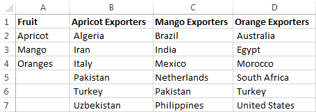
2. Create named ranges
Now you need to create names for your main list and for each of the dependent lists. You can do this either by adding a new name in the Name Manager window (Formulas tab > Name Manager > New) or typing the name directly in the Name Box.
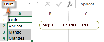
Note. Please pay attention that if your first row is sort of column header like you see in the screenshot above, you shall not include it in the named range.
For the detailed step-by-step instructions please see How to define a name in Excel.
Things to remember:
- The items to appear in the first drop-down list must be one-word entries, e.g. Apricot, Mango, Oranges. If you have items consisting of two, three or more words, please see How to create a cascading dropdown with multi-word entries.
- The names of the dependent lists must be exactly the same as the matching entry in main list. For example, the dependent list to be displayed when "Mango" is selected from the first drop-down list should be named Mango.
When done, you may want to press Ctrl+F3 to open the Name Manager window and check if all of the lists have correct names and references.
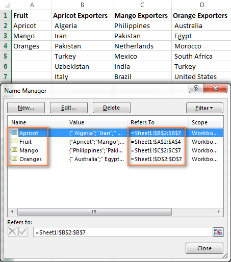
3. Make the first (main) drop-down list
- In the same or in another spreadsheet, select a cell or several cells in which you want your primary drop-down list to appear.
- Go to the Data tab, click Data Validation and set up a drop-down list based on a named range in the usual way by selecting List under Allow and entering the range name in the Source box.
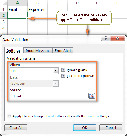
For the detailed steps, please see Making a drop down list based on a named range.
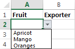
As the result, you will have a drop-down menu in your worksheet similar to this:
4. Create the dependent drop-down list
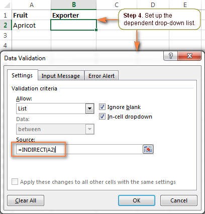
Select a cell(s) for your dependent drop-down menu and apply Excel Data Validation again as described in the previous step. But this time, instead of the range's name, you enter the following formula in the Source field:
=INDIRECT(A2)
Where A2 is the cell with your first (primary) drop-down list.
If cell A2 is currently empty, you will get the error message "The Source currently evaluates to an error. Do you want to continue?"
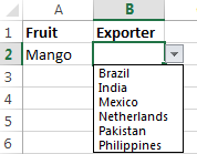
Safely click Yes, and as soon as you select an item from the first drop-down menu, you will see the entries corresponding to it in the second, dependent, drop-down list.
5. Add a third dependent drop-down list (optional)
If needed, you could add a 3rd cascading drop-down list that depends either on the selection in the 2nd drop-down menu or on the selections in the first two dropdowns.
Set up 3rd dropdown that depends on 2nd list
You can make the drop-down list of this type in the same fashion as we've just made a second dependent drop-down menu. Just remember the 2 important things discussed above, which are essential for the correct work of your cascading drop-down lists.
For instance, if you want to display a list of regions in column C depending on which country is selected in column B, you create a list of regions for each country and name it after the country's name, exactly as the country appears in second dropdown lists. For instance, a list of Indian regions should be named "India", a list of Chines regions - "China", and so on.
After that, you select a cell for the 3rd dropdown (C2 in our case) and apply Excel Data Validation with the following formula (B2 is the cell with the second drop-down menu that contains a list of countries):
=INDIRECT(B2)
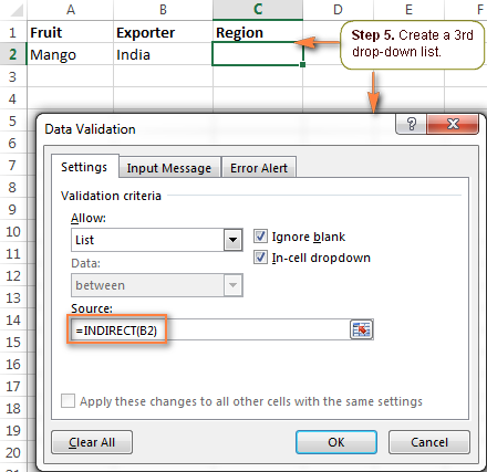
Now, each time you select India under the list of countries in column B, you will have the following choices in the third drop-down:
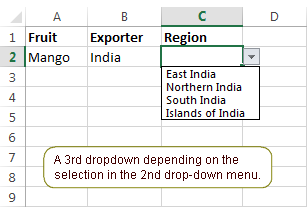
Note. The displayed list of regions is unique for each country but it does not depend on the selection in the first drop-down list.
Create a third dropdown dependent on the first two lists
If you need to create a cascading drop down menu that depends on the selections both in the first and second drop-down lists, then proceed in this way:
- Create additional sets of named ranges, and name them for the word combinations in your first two dropdowns. For example, you have Mango, Oranges, etc. in the 1st list and India, Brazil, etc. in the 2nd. Then you create named ranges MangoIndia, MangoBrazil, OrangesIndia, OrangesBrazil, etc. These names should not contain underscores or any other additional characters.
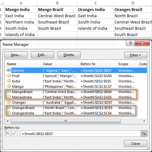
- Apply Excel Data Validation with the INDIRECT SUBSTITUTE formula that concatenates the names of the entries in the first two columns, and removes the spaces from the names. For example, in cell C2, the data validation formula would be:
=INDIRECT(SUBSTITUTE(A2&B2," ",""))Where A2 and B2 contain the first and second dropdowns, respectively.
As the result, your 3rd drop-down list will display the regions corresponding to the Fruit and Country selected in the first 2 drop-down lists.
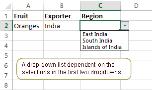
This is the easiest way to create cascading drop-down boxes in Excel. However, this method has a number of limitations.
Limitations of this approach:
- The items in your primary drop-down list must be one-word entries. See how to create cascading drop-down lists with multi-word entries.
- This method won't work if the entries in your main drop-down list contain characters not allowed in range names, such as the hyphen (-), ampersand (&), etc. The solution is to create a dynamic cascading dropdown that does not have this restriction.
- Drop-down menus created in this way are not updated automatically i.e. you will have to change the named ranges' references every time you add or remove items in the source lists. To get over this limitation, try making a dynamic cascading drop down list.
Create cascading drop-down lists with multi-word entries
The INDIRECT formulas that we used in the example above can handle one-word items only. For example, the formula =INDIRECT(A2) indirectly references cell A2 and displays the named range exactly with the same name as is in the referenced cell. However, spaces are not allowed in Excel names, which is why this formula won't work with multi-word names.
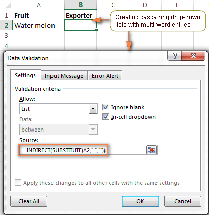
The solution is to use the INDIRECT function in combination with SUBSTITUTE like we did when creating a 3rd dropdown.
Suppose you have Water melon among the products. In this case, you name a list of water melon exporters with one word without spaces - Watermelon.
Then, for the second dropdown, apply Excel Data Validation with the following formula that removes the spaces from the name in cell A2:
=INDIRECT(SUBSTITUTE(A2," ",""))
How to prevent changes in the primary drop down list
Imagine the following scenario. Your user has made the selections in all of the drop-down lists, then they changed their mind, went back to the first list, and chose another item. As the result, the 1st and 2nd selections are mismatched. To prevent this from happening, you may want to block any changes in the first drop-down list as soon as a selection is made in the second list.
To do this, when creating the first dropdown, use a special formula that will check whether any entry is selected in the second drop down menu:
=IF(B2="", Fruit, INDIRECT("FakeList"))
Where B2 contains the second dropdown, "Fruit" is the name of the list that appears in the first drop-down menu, and "FakeList" is any fake name that does not exist.
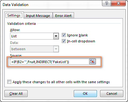
Now, if any item is selected in the 2nd drop-down list, no choices will be available when the user clicks on the arrow next to the first list.
Creating dynamic cascading drop-down lists in Excel
The main advantage of a dynamic Excel dependent drop-down list is that you are free to edit the source lists and your drop-down boxes will get updated on the fly. Of course, creating dynamic dropdowns requires a bit more time and more complex formulas, but I believe this is a worthy investment because once set up, such drop-down menus are real pleasure to work with.
As with almost anything in Excel, you can achieve the same result in several ways. In particular, you can create a dynamic dropdown using a combination of OFFSET, INDIRECT and COUNTA functions or a more resilient INDEX MATCH formula. The latter is my preferred way because it provides numerous advantages, the most essential of which are:
- You have to create 3 named ranges only, no matter how many items there are in the main and dependent lists.
- Your lists may contain multi-word items and any special chars.
- The number of entries can vary in each column.
- The entries' sort order does not matter.
- Finally, it's very easy to maintain and modify the source lists.
Okay, enough theory, let's get to practice.
1. Organize your source data in a table
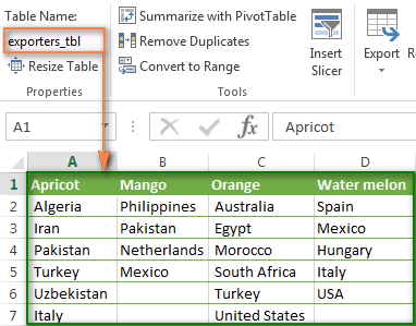
As usual, the first thing for you to do is to write down all the choices for your drop-down lists in a worksheet. This time, you will have store the source data in an Excel table. For this, once you have entered the data, select all of the entries and press Ctrl + T or click Insert tab > Table. Then type a name of your table in the Table Name box.
The most convenient and visual approach is to store the items for the first drop-down as table headers, and the items for the dependent dropdown as table data. The screenshot below illustrates the structure of my table, named exporters_tbl - the fruit names are table headers and a list of exporting countries is added under the corresponding fruit name.
2. Create Excel names
Now that your source data is ready, it's time to set up named references that will dynamically retrieve the correct list from your table.
2.1. Add a name for the table's header row (main dropdown)
To create a new name that references the table header, select it and then either click Formulas > Name Manager > New or press Ctrl + F3.
Microsoft Excel will use the built-in table reference system to create the name of the table_name[#Headers] pattern.
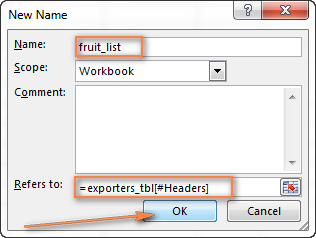
Give it some meaningful and easy to remember name, e.g. fruit_list, and click OK.
2.2. Create a name for the cell containing the first drop-down list
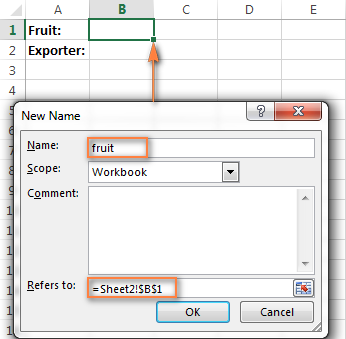
I know that you don't have any dropdown yet :) But you have to choose the cell to host your first dropdown and create a name for that cell now because you will need to include this name in the third name's reference.
For example, my first drop-down box is reside in cell B1 on Sheet 2, so I create a name for it, something simple and self-explanatory like fruit:
Tip. Use appropriate cell references to copy drop-down lists across the worksheet.
Please be sure to read the following few paragraphs carefully because this a very useful tip you that don't want to miss. Thanks a lot to Karen for posting it!
If you plan to copy your drop-down lists to other cells, then use mixed cell references when creating the name for the cell(s) with your first drop-down list.
For the drop-downs to copy correctly to other columns (i.e. to the right), use relative column (without the $ sign) and absolute row (with $) references like = Sheet2!B$1.
As the result, B1's dependent drop down list will appear in cell B2; C1's dependent drop-down will display in C2, and so on.
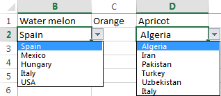
And if you plan to copy the dropdowns to other rows (i.e. down the column), then use absolute column (with $) and relative row (without $) coordinates like = Sheet2!$B1.
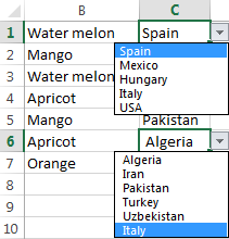
To copy a drop-down cell in any direction, use a relative reference (without the $ sign) like = Sheet2!B1.
2.3. Create a name to retrieve the dependent menu's entries
Instead of setting up unique names for each of the dependent lists like we did in the previous example, we are going to create one named formula that is not assigned to any particular cell or a range of cells. It will retrieve the correct list of entries for the second dropdown depending on which selection is made in the first drop-down list. The main benefit of using this formula is that you won't have to create new names as you add new entries to the first drop-down list - one named formula covers them all.
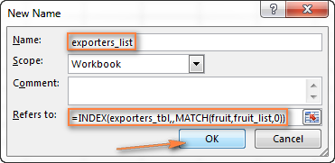
You create a new Excel name with this formula:
=INDEX(exporters_tbl,,MATCH(fruit,fruit_list,0))
Where:
exporters_tbl- the name of the table (created in step 1);fruit- the name of the cell containing the first drop-down list (created in step 2.2);fruit_list- the name referencing the table's header row (created in step 2.1).
I gave it a name exporters_list, as you see in the screenshot below.
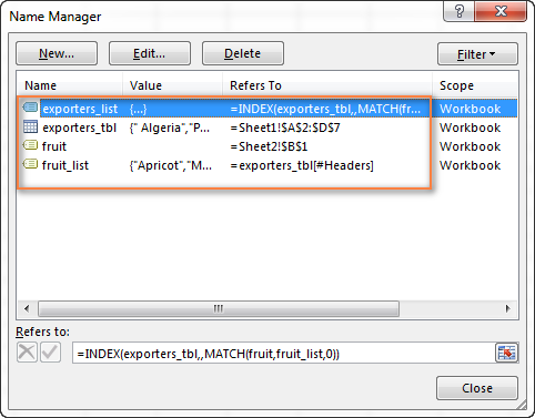
Well, you have already done the major part of the work! Before getting to the final step, it may be a good idea to open the Name Manager (Ctrl + F3) and verify the names and references:
3. Set up Excel Data Validation
This is actually the easiest part. With the two named formulas in place, you set up Data Validation in the usual way (Data tab > Data validation).
- For the first drop-down list, in the Source box, enter =fruit_list (the name created in step 2.1).
- For the dependent drop-down list, enter =exporters_list (the name created in step 2.3).
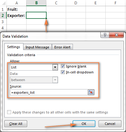
Done! Your dynamic cascading drop-down menu is accomplished and will update automatically reflecting the changes you've made to the source table.
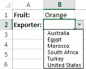
This dynamic Excel dropdown, perfect in all other respects, has one shortcoming - if the columns of your source table contain a different number of items, the blank rows will appear in your menu like this:
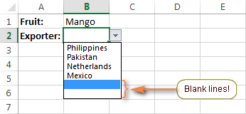
Exclude blank rows from the dynamic cascading dropdown
If you want to clean any blank lines in your drop-down boxes, you will have to take a step further and improve the INDEX / MATCH formula used to create the dependent dynamic drop-down list.
The idea is to use 2 INDEX functions, where the first gets the upper-left cell and the second returns the lower-right cell of the range, or the OFFSET function with nested INDEX and COUNTA. The detailed steps follow below:
1. Create two additional names
Not to make the formula too bulky, create a couple of helper names with the following simple formulas first:
- A name called col_num to reference the selected column number:
=MATCH(fruit,fruit_list,0) - A name called entire_col to reference the selected column (not the column's number, but the entire column):
=INDEX(exporters_tbl,,col_num)
In the above formulas, exporters_tbl is your source table's name, fruit is the name of the cell containing the first dropdown, and fruit_list is the name referencing the table's header row.
2. Create the named reference for the dependent dropdown
Next, utilize either of the below formulas to create a new name (let's call it exporters_list2) to be used with the dependent drop-down list:
=INDEX(exporters_tbl,1,col_num) : INDEX(exporters_tbl, COUNTA(entire_col), col_num)
=OFFSET(INDEX(exporters_tbl,1,col_num),0,0,COUNTA(entire_col))
3. Apply Data Validation
Finally, select the cell containing the dependent dropdown and apply Data Validation by entering = exporters_list2 (the name created in the previous step)in the Source box.
The screenshot below shows the resulting dynamic drop-down menu in Excel where all blank lines are gone!
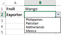
Note. When working with dynamic cascading drop down lists created with the above formulas, nothing prevents the user from changing the value in the first dropdown after making the selection in the second menu, as a result, the choices in the primary and secondary dropdowns may mismatch. You can block changes in the first box after a selection is made in the second one by using either VBA or complex formulas suggested in this tutorial.
This is how you create an Excel data validation list based on the values of another list. Please feel free to download our sample workbooks to see the cascading drop-down lists in action. Thank you for reading!
Practice workbook for download
Cascading Dropdown Sample 1- easy version
Cascading Dropdown Sample 2 - advanced version without blanks
 by
by
319 comments
is there a way for dependent dropdown list without a volatile function?
Why does removing the $ to allow mixed cell reference not allow the second drop down to work? I edited your sample and it broke (named item fruit)
Thanks
Bill
Hi!
When you copy a formula, relative references change. Therefore your dropdown list is using incorrect data. For more information, please visit: Relative and absolute cell reference: why use $ in Excel formula.
I'm getting confused on step 2.3
"You create a new Excel name with this formula:" -- where/how do I do this?
Thank you very much for this guide! It was comprehensive and enabled me to set up several dynamic dependent dropdowns.
Hii..
i have created dependent dropdown for 4 columns using OFFSET function, but problem is that i have same options in third column for all options in second column.
example :
male/female sam hobbies reading
gym
cricket
passion cricketer
Engineer
john hobbies football
swimming
passion writter
football player
sofia hobbies singing
reading
passion singer
for above example i have created dependent dropdown using OFFSET function but in 3rd when i select hobbies or passion it shows only hobbies or passion of sam due to same option names. so when i select john and then hobbies then it should show hobbies of john.
please help me to solve that issue...
I need to create a 3 level dynamic cascading dropdown list. My lists have multi-word entries with special characters and the lists contain a different number of options. I have followed the instructions and can get the first 2 working perfectly, but can't seem to add a third level. For this, I have created a second table, where the header is an exact replica of the second level and tried to reference the 2. I've named the cell in the second column (as in step 2.2), as a reference for the third cell, but all I get in the 3rd dropdown cell (when making an entry) is a blank option.
I have the first 2 levels in one table (as header and table data) as suggested. I don't see how I can include a third level of options using this single table method. Should I create 3 separate tables and what are the steps for this method?
Help!
Hi!
Unfortunately, without seeing your data it is difficult to give you any advice. For the third level of the drop-down list, you need to create a named range. Note that the range name must not contain special characters or spaces. Read more about named ranges in this article.
I'm also looking for a 3rd level.
My data is as follows:
Plan Type -> Carrier -> Product
For example:
In the header row I have my plan types specified then in each column the carriers (and this is working for a 1 level dependency)
A B C
1 ACA Supp PDP
2 Aetna ACE Aetna
3 BCBS Cigna UHC
So, if I select Supp; then I get the option for ACE and Cigna in the next dropdown and based on what I select there, for example, ACE, I would like to have the next dropdown have all of ACE's products (which would be different from Cigna's) and so on.
Thanks for your help!
I'm sorry for the double post - I should have been more specific - I'm using the dynamic cascading drop-down lists method from above and want to have a 3rd tier list based on the answer to the first two since there could be duplication of the company name in the 2nd section - so the unique value would be from the combination of the values in row 1 and the value in, for example, the ACA column. Thanks for any guidance you can provide. Also, the results in the 3rd drop-down would be multiple words with spaces and more than a single option.
For example, if the first drop down is Supp and the 2nd would be Cigna then a selection for the 3rd drop-down could be any of the following:
Plan A
Plan B
Plan C
etc
Or, the options for the 3rd drop-down might be:
Basic health plan
Medium health plan
Super health plan
Super duper health plan
or something like that
Good day
I ram really stuck in trying to do a cascading dependent dropdown list. when using the Offset formula,
1. "=OFFSET($AL$1,1,MATCH($Z3,$AL$1:$AV$1,0)-1,226,1)" this formula in the Data Validation for "List" resulted in it providing the correct drop-down but populating it to ALL the cells below. if I delete the result it also removes the functionality for the next corresponding drop-down selection.
2. I the used the Name Manager (which I can't recall which one) and it worked, BUT when copying to dependent drop-down cells to the rest of the cells below, it still copied all the names down and if cleared, the functionality was gone too.
3. I also tried to have the tables on a different sheet, but it did not allow it.
At this stage I am so confused and do not know which way forward as I cannot even get the initial drop down to work again - or how to clear range names or Name Manager from the cells , which is probably the cause of the problem. I also could not find the page where I found the Offset formula.
There is also INDIRECT but as I said nothing works.
4. Name Manager: must it be workbook or list?
5. I have used Name Manager to list all the content (2nd drop-down dependent on 1st column) under each Header (First drop-down)
i. Name: (header and 1st drop-down selection)
ii. Value: (the content under the Header/1st dropdown)
iii. Refers to: The current Tab and the Cell range of the content)
iv. Scope: tried both Workbook and list
What I need:
NQF Level (First column) Qualification (2nd Column dependent on 1st column selection)
- NQF_L01 - Mathematical Literacy (AET4), or
- NCert: Intro to Mining and Minerals
- NQF_L10 - DscL Dotor Scientae Chemistry
- Phd: Doctorate Phylosophy, etc,
PLEASE guide me in the right direction as I need to make my tool available for use for the audit we are busy with.
Hello!
You can learn more about Excel names, named ranges and Name manager in this article on our blog.
You may find the example files, links to which you can find at the end of this article, helpful.
Thanks a lot very helpful... but not with figures. :)
I want to create the same but with figures and percentages but it does not work. Is there any difference? Is it possible to do it in excel?
Thanks
Hello!
You can use any Excel data type in the drop down list.
Hi all,
good article and very useful use case. However, I somehow could not replicate it in my MacBook, does excel for Mac has certain limitations in this regard.
I am running into difficulties when referencing the source data which is on another sheet called Master
list: This works with all the data on the same page: (my test page)
=INDIRECT(ADDRESS(2, COLUMN($K$1) + MATCH(I2, $L$1#, 0), 4) & "#")
But when I try and add the data validation to a cell on another tab in the workbook it doesn't work: (note Match(G6 has been updated as that is my new drop down cell)
=INDIRECT("Master list"&ADDRESS(2, COLUMN($K$1) + MATCH(G6, 'Master list'!L1#, 0), 4) & "#")
Can you see where I maybe going wrong ?
Hello!
I think you have incorrectly created a link to another book with the INDIRECT function. I recommend reading this guide: INDIRECT formula to dynamically refer to another worksheet.
For example:
=INDIRECT("'Master list'!"&K1)
I can't check the formula that contains unique references to your workbook worksheets.
Hi,
I want to create a dropdown list with non-unique values. I have 2 groups of candidates, Group 1 and Group 2.
So each candidate is assigned to either group, and I want to be able to select names from that group but it seems like the examples I've come across cater to unique, non-repetitive values?
Hello!
The values in Group 1 and Group 2 may overlap. These are two independent lists.
Is it possible to have a cascading list that will populate information that was provided last year, if no data last year a dropdown list is provided?
I tried to complete this with a cascading list of a vlookup for last years data, however the vlookup does not compute. Is there a way to get the vlookup to compute?
Is there such a thing as the database of information in the Table being too big? I cannot seem to make this work on a large scale, but I did make it work on a much smaller scale. Just wondering.
Hi!
These limits may depend on the system resources of your computer, especially the amount of RAM.
Hi Svetlana / team,
"Creating dynamic cascading drop-down lists in Excel" - you perfectly described my use case!
I was researching for three weeks how to use extract a data validation range from one table, organized into dropdown 1 (=headers) and dropdown 2 (=individual columns). I have to admit while using Excel for two decades, i never was proficient enough for creating more than basic sheets.
VLOOKUP, HLOOKUP, INDEX+MATCH, using helper cells for storing extracted range references... ewww.
Thank you so much for sorting this out for me, really appreciated, have a remaining nice week!
Btw, additional info you might think about adding:
- Excel 365 / Excel Online absolutely want semicolons instead of commas in the published formula: =INDEX(exporters_tbl;;MATCH(fruit;fruit_list;0))
And i have observed this requirement at many other places with formulas too. Not all, though.
- Excel 365 online version does not show empty rows as values, Excel 365 desktop does
Hello!
The use of semicolons / commas in Excel formulas is controlled by the List Separator, set in your Regional Settings. Comma is the default list separator in North America and some other countries. In European countries, comma is reserved for the decimal symbol and the list separator is usually set to semicolon.
Hello. I'm trying to create a drop-down list with the same selections across multiple columns. Per column, I'd like to hide the previous selections specific to individual columns. The issue I'm having is that if I select an entry in the first column, the entry is now hidden in every column, not just the first column. Any advice?
Hello,
I've read through this article quite a few times trying to apply it to my project here but keep running into errors. There may be just too much data to do this within excel but maybe I'm just missing some step. Hopefully someone here will be able to guide me in the right direction.
I've created a database consisting of multiple worksheets where each one represents 1 Year (2000, 2001, 2002... etc.), all the way up to 2021. Within each sheet, a table resides consisting of the same 28 Coloumns with Headers representing Car Manufacturers (BMW, Mercedes.... etc.). In the Rows under each Column Header are the Car Models per that Year.
From this, I'm trying to make 3 dynamic dependent drop-down lists (Year, Car, Model), where the last drop-down list (Model), would be dependent on both previous selections (Year, Car).
Is there a way to create this drop-down list to include and pull the source data from all the worksheets? So that I have just 1 set of drop-down lists?
Hello!
The data you want to include in the drop down list must be located in the same range.
You can combine data from several sheets into one (you can use the Copy Sheets tool). Then find the unique values and place them on a separate sheet (you can use the Duplicate Remover tool). Use these values to create a drop down list.
I hope it’ll be helpful. If something is still unclear, please feel free to ask.
Hi!
So i need to create a dropdown list based on this condition
Sheet 1 Column A, the range of list
Sheet 1 Column B, approval is declared (per row)
Sheet 2 D5, i need a drop down list where only the approved items on Sheet 1 Column A is listed.
If it is not approved, it should not show on the list.
What formula should i write on the data validation?
Is this possible? Can anyone help me? Thanks in advance.
Hi!
Please re-read the article above, it covers your case completely.
Hello,
Kindly help me to add two separate dropdown lists depends on a single dropdown list. For example, Both dropdown menu of State & Delivery time depends on the country dropdown menu.
Country: State: Delivery time:
1:India Mumbai 30days for India.
Odisha
Chennai
2:USA Alaska 90days for the USA.
California
Florida
Hi,
Can I use the SUBSTITUTE function within INDEX & MATCH to create dynamic cascading muti-word dropdowns? I did not see an example of combining these two concepts (please let me know if it is there).
Thanks!
I have 2 Dropdown List with the same options (Included and Excluded) in different sheets. If I select " Included" in one dropdown list, it should also select "Included" on another dropdown list I need VBA code for this.
Hi!
Unfortunately, we cannot help you write VBA code.
Hi All,
This was very helpful, but my data looks as shown below. The issue is I have to create the dropdown sourcing this sheet and not create a separate data sheet with unique values. Could you please advise how i go about this.
Currently, I have created a separate data sheet with only unique values and sourced the data from there.
here is the formula i have used:
OFFSET('Data sheet'!$B$21,1,MATCH($E3,'Data sheet'!$B$21:$AN$21,0)-1,COUNTA(OFFSET('Data sheet'!$B$21,1,MATCH($E3,'Data sheet'!$B$21:$AN$21,0)-1,45,1)),1) . This works but i have to source it form main sheet and not data sheet...
Country State City
India Karnataka Bangalore
India Karnataka Mysore
India Karnataka Mangalore
India Karnataka Davangere
India TN Chennai
India TN Ooty
India TN Kanchi
India TN Salem
USA Florida Tallahassee
USA Florida Tallahassee
USA Florida Jacksonville
USA Florida Orlando
USA California Sacramento
USA California Los Angeles
USA California San Francisco
When making the cascading dropdown lists, you cannot use special characters like / (slash) and even - (hyphen or minus) ! Something to note in the instructions.
Hi,
I was needing to find answer to my question on Data Validation Dynamic Drop-Down List+VLOOKUP. I hope you guys can help me achieve what I want to do.
So I'll start off by describing what I would like to do. I have different sheets I would like to look up data on. I made normal data validation drop down lists for my PHASE, PURPOSE, & SPECs. I added a bit of a twist to the CATEGORY to where is only shows the amount of rows under the certain spec and there not be empty slots. All these work within the first two sheets which is fine.
Now for the problem or solution I need to learn;
I need it to work in the following manner; you select your SPEC, after that the CATEGORY column will display the categories under that SPEC, then your CHOICES column will display the choices under that SPEC+CATEGORY. So every SPEC has it own sheet within the workbook.
I don't know how to make it work to where the CHOICES column displays whatever is in its corresponding sheet. BTW i only added about 15 SPECs its work in progress in case I had to go a different route.
I would greatly appreciate any help on this and if I what I am wanting to do is not Dynamic Data Validation Drop Down List + VLOOKUP let me know or if there is an easier way I am all ears.
Thanks,
Bravo
Hello!
This is a complex solution that cannot be found with a single formula. Without seeing your data it is difficult to give you any advice. If you have a specific question about the operation of a function or formula, I will try to answer it.
I am beginner in excel,
I don't know whether my query will be solved through this method, but first i would like to ask for a solution to a problem that i am facing
i want to create an excel sheet where in a column i just want to add the name of the content and the rate of that content should follow up along with it.
in this manner i do not have to continually look up at the rates once i have put the content on it.
It would be of great help if you could help me find a solution.
Hello,
I created the cascading drop-down list, but when I ask to show me the second dependent list, it shows me the (right) Header but not the list it contains. Please could you help me to find what's wrong with it ? I did follow your procedure step by step though.
Hello!
Unfortunately, without seeing your data it is difficult to give you any advice. Check if you have created a named range for each list.
I created dynamic cascading drop-down lists but I'm not able to prevent changes in the primary drop down list using the following formula
=IF(B2="", Fruit, INDIRECT("FakeList"))
Is there a way to incorporate the above?
Hi,
Sorry, it's not quite clear what you are trying to achieve. Please describe your problem in more detail. It’ll help me understand it better and find a solution for you.
Extremely useful. Thank you.
Svetlana,
Thanks for sharing this just in time!
I am able to design my sheet!
Hi Tulaphart,
Glad to know it worked for you!
BTW, if you are using Excel 365, then you can find a much simpler solution in our new article: Make a dynamic dependent dropdown list in Excel an easy way
I am not that experienced with EXCEL. However I do use it to generate quick prototypes for business applications. I use these prototypes to help extract the detailed functional requirements for the users to feed into the design of the production business system application.
One reoccuring feature is the requirement for a cascading drop down box.
The first "Parent " drop down would be a parts list.
This Parent list could have hundreds of entries for the user to select from.
The second (child) Dropdown box contains the LOT Numbers for all of the products.
Therefore the user first selects the Part Number using the Parent Drop Down BOX,
Then the user will use the second drop down box to select the LOT NUmber.
There are normally only 5 or 6 different LOT Numbers for each of the several hundred Part Numbers.
It seems that the use of the EXCEL OFFSET, MATCH, and INDEX functions just cannot do the job.
(But I am not an expert)
What strategy should I follow to accomplish this.
Trying not to use VBA Macros if possible.
Thank you for any help
Chuck
Hello!
Unfortunately, without seeing your data it is difficult to give you any advice. Please reread the article above, it covers your case completely. Thank you.
Thank you! Finally someone with a solution to my problem!
In data validation my source are digit ( numbers ) ,hence I get error message as "The source currently evaluates an error ",Do you want to continue ? .How to solve it . If the source is a text then it works fine ,but if it is a number it dosn't work.
Hello!
I’m sorry but your task is not entirely clear to me. For me to be able to help you better, please describe your task in more detail. Please specify what you were trying to find, what formula you used and what problem or error occurred. Give an example of the source data and the expected result.
It’ll help me understand it better and find a solution for you. Thank you.
I want nested dropdown list.
Example:
Fruit >Apple
>Grapes
>Mango
Country >India
>US
Hi I would like to create a dependent dropdown list but my data is in this manner and its huge data. I only give 2 deps as example but there is a lot of deps. How can i make a drop down with this where my data in class is dependent on the dep.
Example:
DEPS CLASS
SHOES KIDS
SHOES KIDS
SHOES KIDS
SHOES MEN
SHOES MEN
SHOES WOMEN
SHOES WOMEN
CLOTHING UNISEX
CLOTHING UNISEX
CLOTHING UNISEX
CLOTHING MEN
CLOTHING MEN
CLOTHING WOMEN
CLOTHING WOMEN
Thank you so much if you can help on this.
Hello Mary!
I can’t create a dependent drop-down list for you, because I can’t work with your data. I can only help with advice. But for this, ask a specific question - what is the problem, where the error occurs, which formula does not work.
I have tried to follow the instructions above but am getting an error when I put in the formula for the second drop down(The Source currently evaluates to an error. Do you want to continue?) When I chose a selection in the master list, four out of five selections get no response, but one selection (the second option) then fills in the second drop down with options to choose from.
What may I have overlooked or need to modify in order to get the drop downs to work? Your assistance is greatly appreciated.
Thank You
Hello Lin!
I’m sorry but your task is not entirely clear to me.
For me to be able to help you better, please describe your task in more detail. Please let me know in more detail what formula you used and what problem or error occurred. Give an example of the source data and the expected result. It’ll help me understand it better and find a solution for you. Thank you.
I am trying to create a dropdown with options that will then change the option in the second dropdown. I have five options in the first dropdown. I at first used the =INDIRECT($B$24) and then changed to =INDIRECT(B24) and finally have used =INDIRECT(SUBSTITUTE(B24," ","")) as my options in the first drop down have spaces. As I mentioned in the first comment, when I enter the formula for the second dropdown it gives me an error message, The Source currently evaluates to an error. Do you want to continue?, and I am unable to see four out of five of the options in the second dropdown. The second option, which I have as Inventory, will show in the second dropdown but not any of the rest. I am trying to have a person choose one of the options in the first dropdown, which will then give them a second list to choose options from. Such as with my Inventory, then gives the additional options of (Click to Select), Initiate Rental Agreement, Develop Inventory Management Plan, Create a Par Level, Create a sign-out sheet, Other. Right now the first dropdown is in cell B24 and the second dropdown is B35 on Sheet 1 and my list are on Sheet 2.
Hello Lin!
Here is what I could understand. You have the first drop-down list in cell B24. It consists of 5 positions. The second drop-down list is on the same sheet in cell B35. It works with the formula = INDIRECT($B$24).
Next you need to create named ranges. Their names exactly match the values from the first drop-down list. This is described in detail in the manual above. Read it carefully. If you do not, then the second drop-down list will not work.
Perhaps this is the cause of the problem.
No sir, it does not work with any of the formulas. Currently only the second option in my first drop-down will bring anything up in the second drop-down. I currently have the formula =INDIRECT(SUBSTITUTE(B24," ","") as my first drop-down consist of Infection Control, Inventory, Procedure or Protocol, Site or Facility Need, Staffing Shortage. As for the named ranges, yes I have created the named ranges to match the names with the space changed to an _, such as for Infection Control the named range is Infection_Control or for Procedure or Protocol as Procedure_or_Protocol.
Hello Lin!
I do not see your data. Therefore, I can’t name the exact reason. However, remember that the names of your items from the drop-down list must exactly match the names of the named ranges. If the name is "Procedure or Protocol", and the named range is "Procedure_or_Protocol" - this is 100% not working.
Good Evening Alexander. If I'm not mistaken a named range can't have spaces, so how do I make the items in the drop-down match exactly with the named ranges. I was of the understanding that the _ represented a space. How else can I make this work? Would it be better for me to send a copy to you to look at the data or is there another option? I appreciate your time and assistance with this matter.
Hello Lin!
Items in the drop-down list must contain _ instead of a space For instance, Procedure_or_Protocol. Your items from the drop-down list must exactly match the names of the named ranges.
I hope this will help
Is it possible to create a dropdown menu that will automatically fill column A, B, C & D? Basically, I need to make one selection, and have the first four columns autofill.
Thank you!!!! This was a blessing and helped so much!!!!!
Nice article, but stuck. I have a drop down (master) that needs to change three other cells once you change the drop down.
Ex. Historical list A_L, I_N, X_R, R_T
Hours/tops 174, 47.2, 88.3, 13.2
Metric Type Joy, Rain, Sun, Sad
Source Joy.xls, Rain_GL.xls, Sun_2020.xls, Sad.doc
If Historical List changes A_L to X_R
The other need to go from A_L, 174, Joy, Joy.xls to X_R, 88.3, Sun,Sun_2020.xls
I tried making the first Historical List the primary, and the others customer with a =if(B3=C7:C11,D77:D11,0) where B3 = Cell that changes from any given C7-C11 cells (array) and the D column hours/tops. I didn't continue because that didn't work. I tried various others ways, and I am just frustrated.
Hello Kristy!
I'm sorry, it is not very clear what result you want to get. Could you please describe your task in more detail and send us a small sample workbook with the source data and expected result to support@ablebits.com? Please shorten your tables to 10-20 rows/columns and include the link to your blog comment.
We'll look into your task and try to help.
Thanks Svetlana.. though this article was little bit tricky but i have enjoyed it..
hi, is it possible to show 2 named ranges together using data validation. For example list A list of fruits and list B has list of vegetables. in dependent drop down list. we can get if A1 has fruits then List A, and if A1 has Vegetables then List B.
But if A1 = c , i want to the list of both list A and list B, is it possible to do without creating named range including both list.
A question already asked but I didn't find a response ...
Is there a way to automatically update the exporter cell to the first item in the list once the fruit is selected?
i have a problem that is difficult to explain but may well be very easy to solve, my biggest constraint in what i am trying to achieve is that macro is not allowed to be used as the template i am creating is uploaded into a platform that cant accept macros.
Having said that, this is what i want to do: I am using a dependent dropdown list so when i select a particular cell in (column A) with a list, that selection informs another cell adjacent in Column B (another dropdown list) only certain value is available for selection list. I want now to complicate it further because i want to add another dropdown list in column C with a selection of A, B, C etc and hope that when i select A, B or C it will concatenate the data in column B cell. To explain it better, if i select Column A (fruit) Column B list would contain Apple, Pear, Plum, Orange but what if i want to identify the colour of the fruits i would have the colours available in Column C; red, blue, green and pink, so i want to have the option of adding the colours to the fruits in Column B cell.
Thanks a lot! Great tutorial, especially for dynamic drop down!!
Hello,
I want to have a dependent list based on multiple selections from the first list. How do i make the second list only show values associated with the multiple values in the first?
Example:
1st list is "categories" and you can select multiple answers ("Arts, Business"). 2nd column would provide drop-downs for both "Arts, Business" ("design" (within "arts"), "investing"(within "business").
Another example:
List A
A1 "X"
A2 "X1"
A3
Multi-select A1 and A2
Show values with X and X1 to multi-select.
Hi,
Im trying to create a dependent dropdown where the secondary dropdown elements can come multiple types based on primary selection. Eg: If primary dropdown is Apple, Orange and Grapes and second dropdown is China, Brazil and Australia. If I select Apple - say Australia and Brazil should come and I select Orange it should again populate to China and Australia. Is there any way of doing this as creating a range table for every single dropdown is a tedious task and doesnt work with long dropdowns?
I believe there is an easier way to prevent user from changing the value in the first dropdown after making the selection in the second menu (i.e. to prevent mismatches in choices in the primary and secondary dropdowns), easier than the other tutorial linked and definitely easier than VBA:
You can block changes in the first box (or, at least, force the user to clear the second selection before toggling the first dropdown again): changing the formula for the first drop down to =IF(B2="",fruit_list,INDIRECT("fakerange")), as suggested for the simple formula.
For UX, I added a comment to the B2 column header in my actual working sheet (not my data validation sheet) that says "To change the fruit of a line item, first clear the selection in column C by selecting the 'Exporter' chosen, then hit 'delete'". That way, you prevent mismatches, allow the flexibility for changes, empower the user to work autonomously, AND simplify your work considerably. It won't work in EVERY circumstance, but in most, I think this is a much simpler solution.
scrolling toolbar is quite obnoxious. copied/pasted the text I wanted to Word and then went elsewhere. seriously...
what if I have like 3 in the first list, 8 in the second list and 5 in the last list
BUT
I have around 705 total projects
will I need to create a 3x8x5x705= 84 600 data in total for it to work?
I can't even pay attention to the content of the article because of the scrolling ad at the bottom of the screen that makes me nauseous.
Hi, I am having an issue in indirect function. I have used name range method and the drop down works to pick up value from the the list. It works and drop-down list show correctist for first row. When I copy down the rows with fuction for entry, the drop-down does not give the correct referenced list and show list from one row above of the actual referenced cell.
=INDIRECT($A$2). It should pick actually from row 3 which is like =INDIRECT($A$3)
Grateful if anyone can help me on it.
Thanks alot
Michel
Hi Michel,
Using $ ties the indirect function to that cell alone
instead Use =INDIRECT(A2) and you can then copy down for the next few rows with no issues.
Hi, I have created one spreadsheet, where I am selecting employee ID and based on the employee ID all the data will get populated in other cells. I want to clear all cell value if I change the employee ID. Can any of you help me to get it done.
Thanks in advance