The tutorial explains what ISNUMBER in Excel is and provides examples of basic and advanced uses.
The concept of the ISNUMBER function in Excel is very simple - it just checks whether a given value is a number or not. An important point here is that the practical uses of the function go far beyond its basic concept, especially when combined with other functions within larger formulas.
Excel ISNUMBER function
The ISNUMBER function in Excel checks if a cell contains a numerical value or not. It belongs to the group of IS functions.
The function is available in all versions of Excel for Office 365, Excel 2019, Excel 2016, Excel 2013, Excel 2010, Excel 2007 and lower.
The ISNUMBER syntax requires just one argument:
=ISNUMBER(value)
Where value is the value you want to test. Usually, it is represented by a cell reference, but you can also supply a real value or nest another function inside ISNUMBER to check the result.
If value is numeric, the function returns TRUE. For anything else (text values, errors, blanks) ISNUMBER returns FALSE.
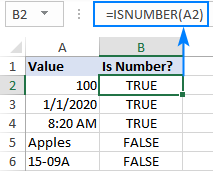
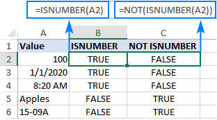
As an example, let's test values in cells A2 through A6, and we will find out that the first 3 values are numbers and the last two are text:
2 things you should know about ISNUMBER function in Excel
There are a couple of interesting points to note here:
- In internal Excel representation, dates and times are numeric values, so the ISNUMBER formula returns TRUE for them (please see B3 and B4 in the screenshot above).
- For numbers stored as text, the ISNUMBER function returns FALSE (see this example).
Excel ISNUMBER formula examples
The below examples demonstrate a few common and a couple of non-trivial uses of ISNUMBER in Excel.
Check if a value is number
When you have a bunch of values in your worksheet and you want to know which ones are numbers, ISNUMBER is the right function to use.
In this example, the first value is in A2, so we use the below formula to check it, and then drag down the formula to as many cells as needed:
=ISNUMBER(A2)
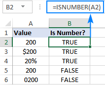
Please pay attention that although all the values look like numbers, the ISNUMBER formula has returned FALSE for cells A4 and A5, which means those values are numeric strings, i.e. numbers formatted as text. There may be different reasons for this, for example leading zeros, preceding apostrophe, etc. Whatever the reason, Excel does not recognize such values as numbers. So, if your values do not calculate correctly, the first thing for you to check is whether they are really numbers in terms of Excel, and then convert text to number if needed.
Excel ISNUMBER SEARCH formula
Apart from identifying numbers, the Excel ISNUMBER function can also check if a cell contains specific text as part of the content. For this, use ISNUMBER together with the SEARCH function.
In the generic form, the formula looks as follows:
Where substring is the text that you want to find.
As an example, let's check whether the string in A3 contains a specific color, say red:
=ISNUMBER(SEARCH("red", A3))
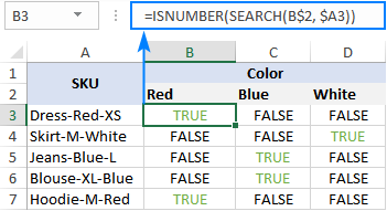
This formula works nicely for a single cell. But because our sample table (please see below) contains three different colors, writing a separate formula for each one would be the waste of time. Instead, we will refer to the cell containing the color of interest (B2).
=ISNUMBER(SEARCH(B$2, $A3))
For the formula to correctly copy down and to the right, be sure to lock the following coordinates with the $ sign:
- In substring reference, lock the row (B$2) so that the copied formulas always pick the substrings in row 2. The column reference is relative because we want it to adjust for each column, i.e. when the formula is copied to C3, the substring reference will change to C$2.
- In the source cell reference, lock the column ($A3) so that all the formulas check the values in column A.
The screenshot below shows the result:
ISNUMBER FIND - case-sensitive formula
As the SEARCH function is case-insensitive, the above formula does not differentiate uppercase and lowercase characters. If you are looking for a case-sensitive formula, use the FIND function rather than SEARCH.
For our sample dataset, the formula would take this form:
=ISNUMBER(FIND(B$2, $A3))
How this formula works
The formula's logic is quite obvious and easy to follow:
- The SEARCH / FIND function looks for the substring in the specified cell. If the substring is found, the position of the first character is returned. If the substring is not found, the function produces a #VALUE! error.
- The ISNUMBER function takes it from there and processes numeric positions. So, if the substring is found and its position is returned as a number, ISNUMBER outputs TRUE. If the substring is not found and a #VALUE! error occurs, ISNUMBER outputs FALSE.
IF ISNUMBER formula
If you aim to get a formula that outputs something other than TRUE or FALSE, use ISNUMBER together with the IF function.
Example 1. Cell contains which text
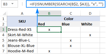
Taking the previous example further, suppose you want to mark the color of each item with "x" like shown in the table below.
To have this done, simply wrap the ISNUMBER SEARCH formula into the IF statement:
=IF(ISNUMBER(SEARCH(B$2, $A3)), "x", "")
If ISNUMBER returns TRUE, the IF function outputs "x" (or any other value you supply to the value_if_true argument). If ISNUMBER returns FALSE, the IF function outputs an empty string ("").
Example 2. First character in a cell is number or text
Imagine that you are working with a list of alphanumeric strings and you want to know whether a string's first character is a number or letter.
To build such a formula, we you'll need 4 different functions:
- The LEFT function extracts the first character from the start of a string, say in cell A2:
LEFT(A2, 1) - Because LEFT belongs to the category of Text functions, its result is always a text string, even if it only contains numbers. Therefore, before checking the extracted character, we need to try to convert it to a number. For this, use either the VALUE function or double unary operator:
VALUE(LEFT(A2, 1))or(--LEFT(A2, 1)) - The ISNUMBER function determines if the extracted character is numeric or not:
ISNUMBER(VALUE(LEFT(A2, 1))) - Based on the ISNUMBER result (TRUE or FALSE), the IF function returns "Number" or "Letter", respectively.
Assuming we are testing a string in A2, the complete formula takes this shape:
=IF(ISNUMBER(VALUE(LEFT(A2, 1))), "Number", "Letter")
or
=IF(ISNUMBER(--LEFT(A2, 1)), "Number", "Letter")
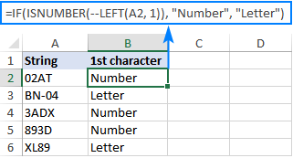
The ISNUMBER function also comes in handy for extracting numbers from a string. Here's an example: Get number from any position in a string.
Check if a value is not number
Though Microsoft Excel has a special function, ISNONTEXT, to determine whether a cell's value is not text, an analogous function for numbers is missing.
An easy solution is to use ISNUMBER in combination with NOT that returns the opposite of a logical value. In other words, when ISNUMBER returns TRUE, NOT converts it to FALSE, and the other way round.
To see it in action, please observe the results of the following formula:
=NOT(ISNUMBER(A2))
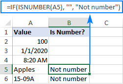
Another approach is using the IF and ISNUMBER functions together:
=IF(ISNUMBER(A2), "", "Not number")
If A2 is numeric, the formula returns nothing (an empty string). If A2 is not numeric, the formula says it upfront: "Not number".
If you'd like to perform some calculations with numbers, then put an equation or another formula in the value_if_true argument instead of an empty string. For example, the below formula will multiply numbers by 10 and yield "Not number" for non-numeric values:
=IF(ISNUMBER(A2), A2*10, "Not number")
Check if a range contains any number
In situation when you want to test the whole range for numbers, use the ISNUMBER function in combination with SUMPRODUCT like this:
For example, to find out if the range A2:A5 contains any numeric value, the formulas would go as follows:
=SUMPRODUCT(--ISNUMBER(A2:A5))>0
=SUMPRODUCT(ISNUMBER(A2:A5)*1)>0
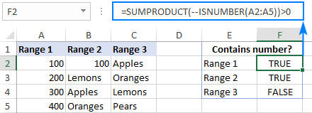
If you'd like to output "Yes" and "No" instead of TRUE and FALSE, utilize the IF statement as a "wrapper" for the above formulas. For example:
=IF(SUMPRODUCT(--ISNUMBER(A2:A5))>0, "Yes", "No")
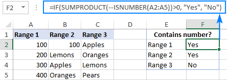
How this formula works
At the heart of the formula, the ISNUMBER function evaluates each cell of the specified range, say B2:B5, and returns TRUE for numbers, FALSE for anything else. As the range contains 4 cells, the array has 4 elements:
{TRUE;FALSE;FALSE;FALSE}
The multiplication operation or the double unary (--) coerces TRUE and FALSE into 1's and 0's, respectively:
{1;0;0;0}
The SUMPRODUCT function adds up the elements of the array. If the result is greater than zero, that means there is at least one number the range. So, you use ">0" to get a final result of TRUE or FALSE.
ISNUMBER in conditional formatting to highlight cells that contain certain text
If you are looking to highlight cells or entire rows that contain specific text, create a conditional formatting rule based on the ISNUMBER SEARCH (case-insensitive) or ISNUMBER FIND (case-sensitive) formula.
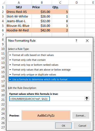
For this example, we are going to highlight rows based on the value in column A. More precisely, we will highlight the items that contain the word "red". Here's how:
- Select all the data rows (A2:C6 in this example) or only the column in which you want to highlight cells.
- On the Home tab, in the Styles group, click New Rule > Use a formula to determine which cells to format.
- In the Format values where this formula is true box, enter the below formula (please notice that the column coordinate is locked with the $ sign):
=ISNUMBER(SEARCH("red", $A2)) - Click the Format button and choose the format you want.
- Click OK twice.
If you have little experience with Excel conditional formatting, you can find the detailed steps with screenshots in this tutorial: How to create a formula-based conditional formatting rule.
As the result, all the items of the red color are highlighted:
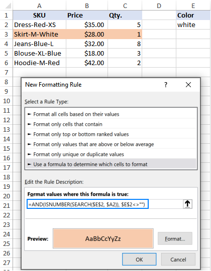
Instead of "hardcoding" the color in the conditional formatting rule, you can type it in a predefined cell, say E2, and refer to that cell in your formula (please mind the absolute cell reference $E$2). Additionally, you need to check if the input cell is not empty:
=AND(ISNUMBER(SEARCH($E$2, $A2)), $E$2<>"")
As the result, you will get a more flexible rule that highlights rows based on your input in E2:
That's how to use the ISNUMBER function in Excel. I thank you for reading and hope to see you on our blog next week!
 by
by
51 comments
I am looking to expand on this Excel Equation. This equation works, but it doesn't put in Past Due for item that are over 6 months. There is an Initial Inspection Date which is column C, list in this format, 2023-11-30 and column N being the column compared to in the format 2023-11 because we only care about the month and year. N1= 2023-11, N2= 2023-06 and N3=2023-07
=IF((ISNUMBER(SEARCH($N$1,$C2))),(IF(ISNUMBER(SEARCH($O$1,$D2)),"Move to In-Process",$D2)),(IF((ISNUMBER(SEARCH($N$2,$C2))),"Move to Close",$D2)))
Is there a way to add the below equation into the above equation to make it work?
(IF((ISNUMBER(SEARCH($N$3,$C2))),"Past Due",$D2))
N3, I have add and is not part of the original table. Can someone help me with figuring out how to expand my equation to put in "Past Due" when the item is over 6 months out from the Initial Inspection Date?
Hi! If I understand the problem correctly, you can add another nested IF function. For more information, please read: Nested IF in Excel – formula with multiple conditions.
=IF((ISNUMBER(SEARCH($N$1,$C2))), IF(ISNUMBER(SEARCH($O$1,$D2)),"Move to In-Process",$D2), IF((ISNUMBER(SEARCH($N$2,$C2))),"Move to Close", IF((ISNUMBER(SEARCH($N$3,$C2))),"Past Due",$D2)))
Hi!
I am trying to find two formulas:
-One that can count if the leftmost character of an entry is any letter or the number 1.
-The other formula should just count entries starting with another number (0, 2, 3, 4, 5, 6, 7, 8, 9; or perhaps just '0')
Do you have any idea how to achieve this?
I am currently using a formula from another post https://www.ablebits.com/office-addins-blog/create-multi-select-dropdown-excel/
with great results, but I can't think of how to implement the above into it.
=SUMPRODUCT(--ISNUMBER(SEARCH("";range))
Rgds
J
Hi! Select the first character from the text string using the LEFT function and check it using this formula:
=SUM((LEFT(A1:A10,1)="1")+(NOT(ISNUMBER(--LEFT(A1:A10,1)))))
HI! I am using the following formula to search for specific number in text, in this case for "65" in cell G8: =IF(ISNUMBER(SEARCH("65",G8)),"65"). The formula, however, tells me also when number 65 is part of different numbers such "165, 650,...". How can i obtain number "65" when "65" stands alone and it is not part of another number? Thank you!
Hi! If your number stands alone, try adding spaces to the search string.
IF(ISNUMBER(SEARCH(" 65 ",G8)),"65")
Hi There
=IF(ISNUMBER(FIND("65",G8)),"65").
how can i include Exclude function in isnumber
I'm looking at using an =if(isnumber(search xx function to search a string which is comments extracted from a database. Doing it when looking for 1 specific entry and having it be a true/false is easy enough.
My issue is, in specific case, am looking for a text reference that hasn't been referred to EXACTLY by everyone (some call it a "PEI", others a "button"), can I have an =if(isnumber with multiple true criteria?
Or do I just run two strings and count separately?
Thankyou!
Hello! If I understand correctly, you can use multiple ISNUMBER in an IF function if you combine them using the logical functions AND or OR.
number length is 10 digits(0773406304), and if stated with "07," replace the 0094 before the 0 in ten digit number
Your number has two digits 0 and no 0094. It is not clear what you want to replace, but try using this guide: Using REPLACE and SUBSTITUTE functions in Excel.
I have data with multiple business types and I need to give each one a number (1-25) - I am using this formula to give the business type restaurant a value
of 1 to pick up any rows with this included.
=IF(ISNUMBER(SEARCH("Restaurant",I2)),"1","2")
Is it possible to give a business type "event" a value of 2 and "takeaway" value of 3 etc etc within the same formula ?
Hi!
For several conditions you can use the nested IF function as described in this article: Nested IF in Excel – formula with multiple conditions.
For example,
=IF(ISNUMBER(SEARCH("Restaurant",I2)),"1",IF(ISNUMBER(SEARCH("event",I2)),"2","3"))
i am trying to have 2 columns on an excel sheet - it is a budget sheet for tenants - i want to have 2 columns one weekly and one monthly.
is there a way to have a formula in each column which will allow user to enter a monthly figure which will then convert into weekly and also if you enter a weekly amount it will convert into the monthly - each time protecting from overwrite.tenants provide some figures weekly and some monthly - im looking a way for entering both sets of data into 2 columns simultaneously - it is not a simple as having one column monhtly then convertin it all to weekly - that i can do.
Any ideas
Hello!
The formulas in your two columns cannot refer to each other, because a circular reference would occur. I think your problem can be solved with VBA.
Hi! I am trying to write a formula with isnumber and could use some help. So far, I have written -
=IF(ISNUMBER(SEARCH($B3,'Sales Skills'!$G5)),'Sales Skills'!$B5,"")
In this scenario, B3 is referencing a cell with text, in this case it's SDE. The problem I'm running into is when I extend the formula to other rows. Later in cell B7, the text is SDET, but the formula seems to be pulling data as if the text in B7 is SDE, I assume because it runs into that answer sooner, and SDE is contained in SDET. Is there a way to change the formula so that it only pulls the specific text in B7? I have too many rows to update the formula to SEARCH("SDET", ... instead of SEARCH($B7 ..
Would really appreciate any help! Thank you!
Hi all
Is there a way to create a forumla to see if the 11 characters match a specific setup e.g.
ABC1234567E
So the first three characters must = ABC then the next 7 must be numbers and the last character = E.
I can work out some of it easy enough e.g. =IF(LEN(H3)="ABC","Ok","Review") but how do i add the rest to this?
Thanks
Hello!
Regular expressions are used to match text strings with a pattern. You can find the examples and detailed instructions here: Regex Match in Excel: regular expression matching with examples.
Use this pattern:
ABC\d{7}E\b
=RegExpMatch(A1, "ABC\d{7}E\b")
How would I create an =ISNUMBER that returns TRUE for a series of Columns, i.e., A3,H3,K3 all contain numbers and are therefore TRUE, and FALSE if there is a column with a blank, i.e., A3 has a number, but H3 and K3 are blank?
Hi!
If I understand your task correctly, try the following formula:
=ISNUMBER(H3)*ISNUMBER(A3)*ISNUMBER(K3)>0
hello,
this is the formula i am using: =FILTER(Table2[ID],NOT(ISNUMBER(MATCH(Table2[ID],Table1[ID],0))),"") i am finding numbers that appear in one column but not the other. currently the numbers in Table2 are as such: 5326_1001200000033566.Table1 column appear as 1001200000033566. is there a way to search by the numbers after the underscore in Table2?
Thanks!
Hello!
To determine partial text matches in cells, use the SEARCH function.
ISNUMBER(SEARCH(B1,A1))
ISNUMBER will return TRUE if there is a partial match B1 and A1.
Thanks so much Alexander!
How do i check for duplicates in a row that contains some text cells and some number cells, but I want to check for duplicates only for the numbers? Thank you
Hello!
To search for duplicates only among numbers, you can use the ISNUMBER function with the formulas described in this article: How to find duplicates in Excel. For example,
=IF(ISNUMBER(A2),COUNTIF(A:A, A2)>1,"")
I hope it’ll be helpful.
I am trying to use the isnumber(search function to filter out numbers 0-10. But when I use the function for ‘1’ it includes all of the ‘1s’ found in the number ‘10’. And all of the ‘0s’ in the ‘10’. How do I overcome this?
Hi!
I recommend comparing numbers as numbers, not as text. I don't know how exactly you are filtering the records. When using the FILTER function, here is an example -
=FILTER(A2:C13, B2:B13=1, "")
Hi
Any idea how can I use ISNUMBER to check if either of the values exists in a cell and then return true or false if the formula found either one of them ?
Currently the formula checks one value, How do I modify it to check more than one value
=IF(ISNUMBER(SEARCH(Sheet10!$A$13,A2)),"YES","NO")
Thanks
Essam
Hello!
Use the SUM function to determine how many values match.
If I understand your task correctly, the following formula should work for you:
=IF(SUM(--(ISNUMBER(SEARCH(A1:A3,B1)))),"Yes","No")
Hi Alexander!
I will explain the task I have:
I have a list of cells that contain data, I need to lookup certain text within each cell and if the text is found I need to categorize the cell, Example:
cell1: barcode app
cell2: QR Scanner app
Categories Index:
QR Apps - QR, barcode
the formula I used works on one cell:
=IF(ISNUMBER(SEARCH(B$3,A2)),"YES","NO") - In this case let's assume the cell B3 contains the word barcode
but whenever I try to add another cell (B3:B4,A2) I get an error.
So I'm trying to cover all the words for each category in one formula, is that possible ?
I appreciate the help
Essam
Hello!
The SEARCH function can only search for one value. For multiple values, you can use an IF OR statement or an IFS function.
=IF(OR(ISNUMBER(SEARCH(B$3,A2)), ISNUMBER(SEARCH(B$4,A2))),"YES","NO")
Hi , i am looking at formula , if start with A then left ( A2,14) if start with P then left (A2,18)
Hi!
To extract the first letter from a text, use the LEFT function. Check this letter for a match using the nested IF function with two conditions.
=IF(LEFT(A1,1)="A",LEFT(A2,14),IF(LEFT(A1,1)="P",LEFT(A2,18),""))
Statement, functions, conditional formatting in excel when using simple functions in a cell then there is no problem to get it to work, but when u want to apply to the whole table in one or more columns then this mostly simply doesn't work. And i know why "proper entry function format" that is cucumber some complicated.
I want to check whole table in multi column from start to end every cell containing whole number against prime number group with a function, and if true then color cell or color number. I can do this in one column at the time only against one number at the time with conditional format function, and that is tedious work to do by hand. I cant figure out how to check against known group prime numbers using conditional format function ! I can define function with no error in it, but simply doesn't work !
Hi!
If I understood the problem correctly, you can write your group of numbers in a separate column of the table and use these guidelines: How to highlight duplicates in a range.
Hope this is what you need.
Number counter KPI
45 a ( 100.0 * ( 1.0 - ( ( 1.0 - ( ( a - b ) / c ) ) * ( 1.0 - ( ( d - e ) / a ) ) ) ) )
33 b ( (b / e ) * 100.0 )
55 c ( e / 1000000.0 )
66 b
77 e
Hi Need help, i want to replay KPIs a,b,c,d,e by 45,33 55,66,77, what formula i can apply
Hi!
What do you want to calculate exactly? Your question is not entirely clear, please specify.
Hi, I want to calculate the KPI, the KPIs are formed with alpha names but in the data model these alpha ref to numeric names which are equal to some value, so I cannot use the KPI formula because the data model doesn't know the KPI formula as is, I need to change the kpi formula to numeric names so the KPI formula will work.
Hi!
The information you provided is not enough to understand your case and give you any advice, sorry. I don't know what KPI is. Explain more simply.
=IF(ISNUMBER(SEARCH($B16,AF$3)),AF$1,"")
What do I need to fix in this formula, it is picking up on partial matches instead of an exact match
Hello!
To determine an exact match, use the methods in this guide: How to compare two cells in Excel.
Please try the following formula:
=IF($B16=AF$3,AF$1,””)
or
=IF(EXACT($B16,AF$3),AF$1,””)
I hope it’ll be helpful.
mango code no.= 01
banana code no.= 02
in a cell alpha numeric no. R25690166 in which fifth and six digit number are code of either banana or mango.
which formula should I use to find out code.
Hi!
To extract the fifth and sixth digits from text, you can use the MID function.
=MID(A1,5,2)
I recommend reading this guide: Excel substring functions to extract text from cell.
Hello!
Is it possible to use isnumber search on an entire column? Currently I am only able to obtain a true match when linking one cell to the other.
Example: I am looking for the number 123456 within a column that contains (John Smith - 0001234560).
As stated, if I link one cell to the correct cell, it works. If I link, one cell to a column - it returns false.
Thanks in advance!
Hi!
You didn't say what result you want. Here are some formulas.
=ISNUMBER(SEARCH("123456",A1:A100))
=SUM(--ISNUMBER(SEARCH("123456",A1:A100)))
If this is not what you wanted, please describe the problem in more detail.
is did posible why does it not work?
B1&IF(OR(ISNUMBER(FIND("TEXT",A1)),ISNUMBER(FIND("TEXT1",A1)),A2,"")
every cel is text i have asked this question some ware but maybe did and up in spam mail who i deleted.
Hello!
You have a mistake in your formula.
=B1&IF(OR(ISNUMBER(FIND("TEXT",A1)),ISNUMBER(FIND("TEXT1",A1))),A2,"")
I want to replace so many jitesh
pls advice
=IF(ISNUMBER(SEARCH("Drumstick PKM 1 50 gm",Q2)),2,IF(ISNUMBER(SEARCH("Bajra No",Q2)),3,IF(ISNUMBER(SEARCH("induce",Q2)),4,IF(ISNUMBER(SEARCH("pusa",Q2)),8,IF(ISNUMBER(SEARCH("ajay",Q2)),9,IF(ISNUMBER(SEARCH("Humic Acid Roota 1 kg",Q2)),10,IF(ISNUMBER(SEARCH("Humic Acid Roota 500 gm",Q2)),11,IF(ISNUMBER(SEARCH("Cucumber",Q2)),12,IF(ISNUMBER(SEARCH("930",Q2)),13,IF(ISNUMBER(SEARCH("latika",Q2)),14,IF(ISNUMBER(SEARCH("2338 250",Q2)),16,IF(ISNUMBER(SEARCH("lucky",Q2)),17,IF(ISNUMBER(SEARCH("bhim",Q2)),18,IF(ISNUMBER(SEARCH("karishma",Q2)),19,IF(ISNUMBER(SEARCH("BAIF",Q2)),21,IF(ISNUMBER(SEARCH("Arka",Q2)),22,IF(ISNUMBER(SEARCH("Alamdar 51",Q2)),23,IF(ISNUMBER(SEARCH("kajol",Q2)),25,IF(ISNUMBER(SEARCH("Bijankur",Q2)),28,IF(ISNUMBER(SEARCH("Auskelp 500 ml",Q2)),29,IF(ISNUMBER(SEARCH("Supplement Vimicon",Q2)),30,IF(ISNUMBER(SEARCH("Aspartical",Q2)),31,IF(ISNUMBER(SEARCH("Lucerne RL88",Q2)),33,IF(ISNUMBER(SEARCH("Okra 2338 100",Q2)),34,IF(ISNUMBER(SEARCH("Subabul",Q2)),35,IF(ISNUMBER(SEARCH("PKM 1 250",Q2)),36,IF(ISNUMBER(SEARCH("Shevari CMS 800",Q2)),37,IF(ISNUMBER(SEARCH("COFS 29 50",Q2)),38,IF(ISNUMBER(SEARCH("COFS 29 200",Q2)),39,IF(ISNUMBER(SEARCH("Agathi 400",Q2)),40,IF(ISNUMBER(SEARCH("Agathi 800",Q2)),41,IF(ISNUMBER(SEARCH("Shevari CMS 400",Q2)),42,0))))))))))))))))))))))))))))))))
sandeep kelkar, Try something like this.
Formula is in cell B1
{TEXTJOIN(", ", TRUE, IF(COUNTIF(A1, "*"&$C$1:$C$7&"*"), $C$1:$C$7, ""))}
A B C
1 I'm looking for Humic Acid Roota 1 kg Humic Acid Roota 1 kg Drumstick PKM 1 50 gm
2 Bajra No
3 pusa
4 ajay
5 Humic Acid Roota 1 kg
6 Humic Acid Roota 500 gm
7 Cucumber
NOTE 1 - You need to press Ctrl + Shift + Enter keys together to get the first result, and then drag the fill handle down to the cells that you want to apply this formula,
NOTE 2 - This formula is only available in Excel 2019 and above.
Good luck.
sandeep kelkar, Please note the info above did not translate properly. The data in the cells should be as follows:
Cell A1 = I’m looking for Humic Acid Roota 1 kg
Cell B1 = Contains the TEXTJOIN formula
Cell C1:C7 Contains the data table containing the following data:
Drumstick PKM 1 50 gm
Bajra No
pusa
ajay
Humic Acid Roota 1 kg
Humic Acid Roota 500gm
Cucumber
I hope this clarifies the situation.
Roy