This tutorial explains how to use the MIN function in Microsoft Excel 2007 - 2019, find the lowest value by a condition and highlight the bottom number in your range.
Today you will learn how to use basic but quite important MIN function in Excel. You'll see the ways to get the lowest number excluding zeroes, the absolute minimum and the smallest value based on some criteria.
Furthermore, I'll show you the steps to highlight the least cell and tell you what to do if your MIN functions return an error instead of the result.
Well, let's get started. :)
MIN function - syntax and usage examples in Excel
The MIN function checks your data range and returns the smallest value in the set. Its syntax is the following:
number1, [number2], … is the series of values from where you want to get a minimum. Number1 is required while [number2] and the following are optional.
There are up to 255 arguments allowed in one function. The arguments can be numbers, cells, arrays of references, and ranges. However, arguments like logical values, text, empty cells are ignored.
Examples of using MIN formula
MIN is one of the easiest functions to apply. Let me prove it to you:
Example 1. Locating the smallest value
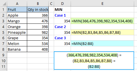
Let's say you have some fruits in stock. Your task is to check if you are running out of any. There are several ways to go:
Case 1: Enter each and every numeral from the Qty in stock column:
=MIN(366, 476, 398, 982, 354, 534, 408)
Case 2: Reference the cells from the Qty column one by one:
=MIN(B2,B3,B4,B5,B6,B7,B8)
Case 3: Or simply reference the whole range:
=MIN(B2:B8)
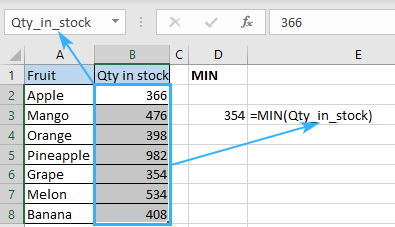
Case 4: Alternatively, you can create a named range and use it instead to avoid any direct references:
=MIN(Qty-in-stock)
Example 2. Looking for the earliest date
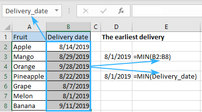
Imagine that you have a few deliveries planned and would like to be ready for the most upcoming one. How to discover the earliest date in Excel? Easy! Use MIN following the same logic from example 1:
Apply the formula and select the dates either by referencing the range directly:
=MIN(B2:B8)
Or the named range:
=MIN(Delivery-date)
Example 3. Retrieving an absolute minimum
Supposing that you have a data range and need to detect not simply the lowest but the absolute minimum there. The MIN alone won't be able to handle that since it will just return the smallest number. Here you need a helper function that can convert all negative numbers to positive ones.
Is there a ready-made solution here? The question was rhetorical, there is a solution for any task in Excel. If you have any doubts, just look through our blog. :)
But let's get back to our task. The ready-made solution to this particular case is called ABS function which returns the absolute value of numbers you specify. Thus, the combination of MIN and ABS functions will do the trick. Just enter the following formula in any blank cell:
{=MIN(ABS(A1:E12))}
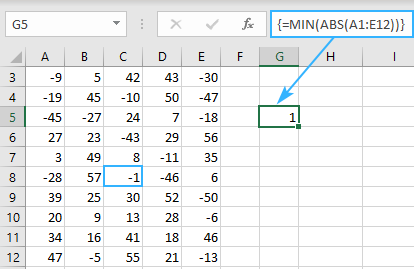
Note! Did you notice the curly brackets around the function? It's a sign that this is an array formula and it needs to be entered via Ctrl + Shift + Enter, not just Enter. You can read more about array formulas and their usage here.
How to find the lowest value ignoring zeros
Does it seem like you know everything about locating the minimum? Don't jump to conclusions, there is plenty left to learn. For example, how would you determine the least non-zero value? Any ideas? Don't cheat and google it, just keep reading ;)
The thing is, MIN works with not only positive and negative numbers but also with zeroes. If you don't want zeros to be that minimum, you need some help from the IF function. Once you add the limitation that your range should be more than zero, the expected result won't keep you waiting. Here is a sample of the formula that returns the bottom value based on some condition:
{=MIN(IF(B2:B15>0,B2:B15))}
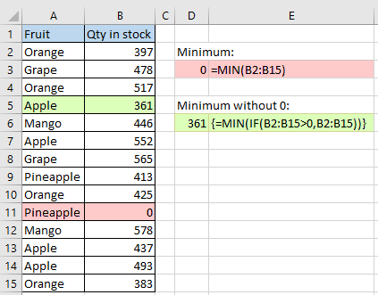
You must have noticed the curly brackets around the array formula. Just remember that you don't enter them manually. They appear one you hit Ctrl + Shift + Enter on your keyboard.
Finding the minimum based on a condition
Let's suppose you need to locate the least sales total of a specific fruit in a list. In other words, your task is to determine a minimum based on some criteria. In Excel, conditions usually lead to using the IF function. All you need to do is make a perfect combination of MIN and IF to solve this task:
{=MIN(IF(A2:A15=D2,B2:B15))}
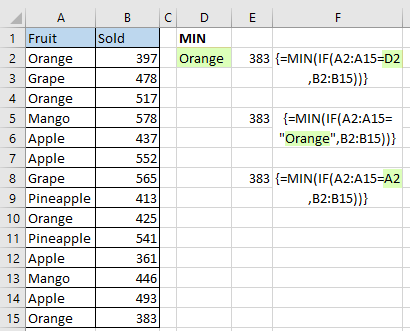
Press Ctrl + Shift + Enter so that array function to work and enjoy.
Looks pretty easy, right? And how will you spot the littlest figure based on 2 or more conditions? How to determine the minimum by multiple criteria? Maybe there is an easier formula available? Please check this article to find it out. ;)
Highlight the smallest number in Excel
And what if you don't need to return the littlest numeral is, but want to find it in your table? The easiest way to guide your eye to this cell is to highlight it. And the most straightforward way to do that is to apply conditional formatting. It's even simpler than writing functions:
- Create a new conditional formatting rule by clicking Conditional formatting -> New Rule
- Once the New Formatting Rule dialog opens, select the “Format only top or bottom ranked values” rule type
- Since the task is to highlight the one and only lowest digit, choose the Bottom option from the drop-down list and set 1 as a quantity of cells to highlight.
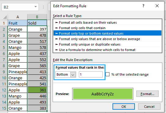
But what to do if there is a zero in your table again? How to ignore zeroes when highlighting the least number? No worries, there is a trick here too:
- Make a new conditional formatting rule selecting the “Use formula to determine which cells to format” option
- Enter the following formula in the Format values where this formula is true field:
=B2=MIN(IF($B$2:$B$15>0,$B$2:$B$15))
Where B2 is the first cell of the range to highlight the lowest number in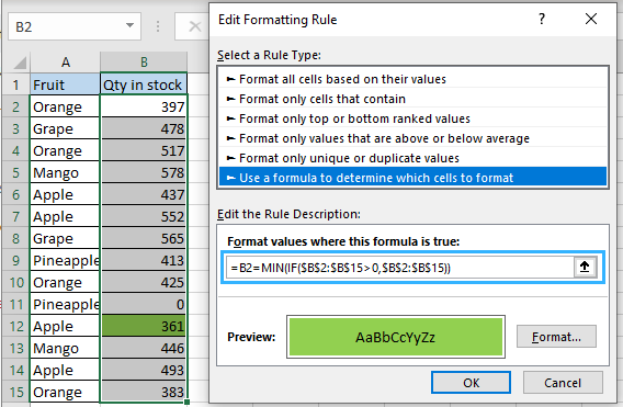
- Set the color (Edit Formatting rule -> Format… -> Fill) and hit OK.
- Enjoy :)
Tip. To find the Nth lowest number with criteria, use the SMALL IF formula.
Why doesn't my MIN function work?
In the ideal world, all the formulas would work like a charm and return the correct results once you hit Enter. But in the world we live in it happens that functions return an error instead of the result we need. No worries, the error itself always hints at its possible cause. You just need to have a closer look at your functions.
Fixing the #VALUE error in MIN
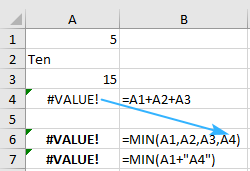
Generally, you get the #VALUE! error message when at least one of the arguments used in a formula is incorrect. Regarding MIN, it may occur when one of them is corrupted e.g. something is wrong with the data the formula refers to.
For instance, #VALUE! may appear if one of its arguments is a cell with an error or there is a typo in the its reference.
What can cause the #NUM! error?
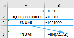
Excel shows a #NUM error when it is impossible to calculate your formula. It usually takes place when the numeric value is too big or small to be displayed. The allowed numbers are those between -2.2251E-308 and 2.2251E-308. If one of your arguments is outside this scope, you'll see #NUM! error.
I'm getting #DIV/0! error, what to do?
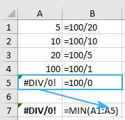
Fixing #DIV/0! is easy. Don't divide by zero! :) No kidding, this is the one and only solution to that issue. Check if there is a cell with #DIV/0! in your data range, fix it and the formula will return the result right away.
Looking for the littlest numeral but getting the #NAME? error?
The #NAME error means that Excel can't recognize the formula or its arguments. The most possible reason of such a result is a typo. You may either misspell the function or put incorrect arguments. Moreover, text representations of numbers will cause that error too.
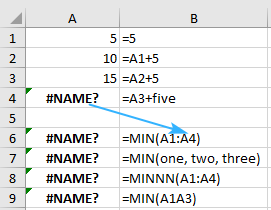
The other possible cause of that problem lays in a named range. So, if you reference an unexisting range or there is a typo in it, you'll see #NAME? in the place you're expecting your result to appear.
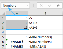
These are the ways to find a minimum using the Excel MIN function. For you, I covered different approaches to discover the lowest value and to locate the absolute minimum. You may consider this your cheat sheet and use it whenever you need to get the smallest number based on a condition and to prevent and fix the possible errors.
That's it for today. Thank you for reading this tutorial! Please feel free to share your thoughts and questions in the comments section, I'll be glad to get feedback from you! :)
 by
by
40 comments
Hi
I posted earlier with a query re Min function but on reading it back realised that I did not make it clear.
I would like to find a specific time in a range and then count back the cells. The time may not be the minimum. It would be the time that I enter in a cell apart from the range.
(The formula would be used in a greyhound / horse racing programme. I have tried but cannot sort this problem. Ok with Min in range but have difficulty with the specific time and then count back the no of runs.) Hope this is clear enough.
Thanks in anticipation
Alex
Hi
Could you help if poss
I would like to find a time in a range that is the minimum time and count back the no of cells in that range.
(Its actually for a greyhound racing formula where I would like to record the no of runs back that the best time was achieved)
thanking you in anticipation
Alex
Hi! If I understand correctly, try the MATCH function to find the number of position of the minimum value.
=COUNT(A1:A10)-MATCH(MIN(A1:A10),A1:A10,0)
ANIMALS QNTY
DOG 2
CAT 3
COW 5
DOG 2
CAT 4
COW 2
RAT 6
RABBIT 1
I have this kind of table and i need here Name the animal which is MIN Qnty.
Hi! Find the minimum value with the MIN function and use it in the INDEX MATCH search.
=INDEX(A2:A20,MATCH(TRUE,MIN(B2:B20)=B2:B20,0))
Hope this is what you need.
Hi,
Thank you. I'm looking for this but i need to avoid blank cell.
Sorry its avoid blank cell.
Hi! I wrote this formula based on the description you provided in your original comment. Please note that if you’d provided me with the precise and detailed description of your task from the very beginning, I’d have created a different formula that would have worked for your case.
However, this formula ignores empty cells in column B. Describe the problem in detail.
Hi,
Kindly assist me on how to code formular usinf VBA on the cell.
Column A is minute of day; Column B is temperature. In Columns C and D, would like to return minimum temperature and minute of that temperature.
Min function returns the minimum temp. How do I return the minute of that minimum temperature?
Thank you.
Hi! Use INDEX MATCH function. You can find the examples and detailed instructions here: Excel INDEX MATCH vs. VLOOKUP - formula examples. Try this formula:
=INDEX(A1:A20,MATCH(TRUE,B1:B20=MIN(B1:B20),0))
Hello
I'm trying to find the minimum value of C3:C372 >$100 if A3:A372 = MON. I'm struggling with any sort of format that I have tried. Your help would be appreciated
Hello!
You can find a conditional minimum value with the MINIFS function. You can find the examples and detailed instructions here: How to use MINIFS function in Microsoft Excel.
The formula might look like this:
=MINIFS(C3:C372,C3:C372,">100",A3:A372,"MON")
Thank you so much
I need a formula to get the minimum login time (located in COLUMN E) for column E only if the IDs match in column B and K(IDs in column K to match Those in column B). Here is the formula I'm using: =MIN(IF(K2=$B$2:$B$76,$E$2:$E$76,MAX($E$2:$E$76))).
This formula gives me a zero though it works in other sheets with the same type of data and formats.
I am working with two worksheets. sheet 1 to calculate the data in sheet 2.
I am trying to return the oldest date (ignoring zeros or blanks) in column H of sheet2, if column O of sheet2 matches Column A of sheet1.
Example
Sheet 1
Column A
tp-2201
tp-2202
tp-2203
Sheet 2
Column H
07/01/2022
09/25/2022
blank
Sheet 2
Column 0
tp-2201
tp-2202
blank (source had nothing to return for this inventory, so it doesnt exist in the list on sheet2)
i am looking to have the formula in place on Sheet 1, should the list on Sheet 2 contain tp-2203 the next day. I am looking to have the formula return a blank if there is nothing to report for that item.
I hope that makes sense.
I am currently using this formula, which does return oldest date.
=MIN(IF(Sheet2!O1#=A4,(Sheet2!$H:$H)))
How do I then get the formula to return a blank cell when there is nothing to return, rather than getting "01/00/1900"
I figured it out!
=IF(MIN(IF(Sheet2!O1#=A4,(Sheet2!$H:$H))) > 0, MIN(IF(Sheet2!O1#=A4,(Sheet2!$H:$H))), "")
I'm using =MIN(A1:A50,B1:B50) as an example. Getting the min of of either set, whichever is the lowest as expected!
Can I conditional format the result by Text color somehow, so that I can know what set the result is from?
Thanks
Hello!
If I understand your task correctly, to highlight the minimum value, you can use conditional formatting with the formula –
=(A1=MIN(A1:A50,B1:B50))*(A1:B50<>"")
Hope this is what you need.
New example:
Data range A1:A20 was font color Blue, and data range B1:B20 was font color red.
And formula =MIN(A1:A20,B1:B20) was in Cell C1,
Is it posable to conditional format C1 with a formula that would return its value in either Red or Blue based on what Data range the result came from (either Red or blue text color in C1)
Thanks again!
Hi!
A conditional formatting rule can only set one color.
How do i find the minimum age per district in a dataset with demographics of people from different districts in excel. The district and ID number are combined so i want to pick out the district without creating a different field
Hi!
Sorry, I do not fully understand the task. Please give me with an example of the source data and the expected result.
i'M TRYING TO EXTRACT THE LOWEST NUMBER IN COLUMN B , RANGE B1:B21 CONTAINING DECIMAL NUMBERS FROM (-10 TO +10); COLUMN A ARE NAMES. WHEN I USE MIN(B1:B21) RESULTS IN "0" INSTEAD OF "-10" WHICH WAS THE LOWEST.
THANK YOU FOR YOUR HELP
Hi!
I have not been able to reproduce your problem. I can assume that your numbers are written as text. Check it.
Good afternoon,
I am getting "You've entered too many argument for this function." This is what I am trying to do. I have 10 numbers in different cell columns (not all cell have numbers).
A1=25 A2=30 A3=$ sign A4=35 A5=blank A6=40 A7=0 (zero) A8=45 A9=50 & A10=55
When I use this formula =MIN(IF(A1,A2,A3>0)), I get no errors. However, as soon as I add more cells or all 10 cell, I get the "too many argument" error. I can't use (A1:A10) because there are cells that I do not want to be included.
Is there a different formula that I can use to find the 1st lowest, 2nd lowest, and 3rd lowest to show on cell A11?
Thanks in advanced
Hello!
To find the N smallest values, you can use the SMALL function. But you can't look at individual cells, only a range. To find the smallest values by condition, use this guide: How to find smallest values ignoring zeros.
=SMALL(IF(A1:A10<>0,A1:A10),1)
I hope I answered your question. If something is still unclear, please feel free to ask.
Good morning,
Thanks again for your reply. I had to rearrange my data so I could use the range method. The issue I have now is in some cells there are no value yet. They have a $ symbol. I want to have the formula setup before data are entered.
A B
Row1 Tom $25
Row2 Jerry $50
Row3 Micky $
Row4 Jane $15
When I use your formula =SMALL(IF(B1:B4,0,B1:B4),1) I get an error. What I would like to be able to do is to have this formula return the person's name with the lowest value, ignoring zero and symbols.
Thanks in advanced,
Hello!
This formula returns the smallest value, ignoring zero and character values.
=SMALL(IF(B1:B10<>0,B1:B10),1)
To get the corresponding value from column A, use the INDEX+MATCH formula
=INDEX(A1:A10,MATCH(SMALL(IF(B1:B10<>0,B1:B10),1),B1:B10,0))
This should solve your task.
Hello, I am trying to do something similar, not ignore a text field when no data is given in a column.
EG: AGE 25, 42, 51, NAG, 34, 47, etc
My MAX formula works well... =MAX(IF(ISNUMBER($G$2:$G$14000),$G$2:$G$14000))
But my MIN formula returns a minus value of -972 ???
=MIN(IF(ISNUMBER($G$2:$G$14000),$G$2:$G$14000))
Any suggestions would be appreciated, and thanks for your help in advance.
Sorry, just to clarify:
Column G contains the ages and the 'NAG' ('no age given' text)...
AGE: 25, 42, 51, NAG, 34, 47, etc
Hello!
I've tried using your formula in my sample workbook and it worked like a charm. It looks like there is a cell with -972 somewhere in your range of search. You may try and use Find and Replace (Ctrl+F) to locate it in your spreadsheet.
Hi Alexander - thank you for that - I tried the Find & Replace - but couldn't locate the error - so i ran a =IF(G2<0,G2,"") formula down the length of the columns to locate the one negative number, and it suddenly appeared - FIXED! and it all works perfectly now - cheers and thank you sooooooo much!
Hello
i'd like to extract the supplier with the lowest price (except zero) in this example. appreciate your help
supplier#1 supplier#2 supplier#3 RESULT
sku001 $4.85 $3.85 $1.85 supplier#3
thank you
Hello!
If I understand your task correctly, the following formula should work for you:
=INDEX($A$1:$C$1,IF(SMALL(A2:C2,1)>0, MATCH(SMALL(A2:C2,1),$A$2:$C$2,0), MATCH(SMALL(A2:C2,2),$A$2:$C$2,0)))
I hope this will help
I am using a MIN function that seems to work in simple spreadsheet and the same function when applies in other returns the answer as 0 when it shouldn't. I use the evaluate formula and can clearly see it should be a number bigger than 0, but the answer comes out as 0. Any suggestions on what the issues maybe there?
Hello!
For me to be able to help you better, please describe your task in more detail. It’ll help me understand it better and find a solution for you. Thank you.
=IF(D9>=15,C10=15,C10=D9)
Formula in C10:
=IF(D9>=15,15,D9)
Did I guess correctly?