The tutorial shows how to use the CELL function in Excel to retrieve various information about a cell such as cell address, contents, formatting, location, and more.
How do you usually get specific information about a cell in Excel? Someone would check it visually with their own eyes, others would use the ribbon options. But a faster and more reliable way is to use the Excel CELL function. Among other things, it can tell you whether a cell is protected or not, bring a number format and column width, show a full path to the workbook that contains the cell, and a lot more.
Excel CELL function - syntax and basic uses
The CELL function in Excel returns various information about a cell such as cell contents, formatting, location, etc.
The syntax of the CELL function is as follows:
Where:
- info_type (required) - the type of information to return about the cell.
- reference (optional) - the cell for which to retrieve information. Typically, this argument is a single cell. If supplied as a range of cells, the formula returns information about the upper left cell of the range. If omitted, the information is returned for the last changed cell on the sheet.
Info_type values
The following table shows all possible values for the info_type argument accepted by the Excel CELL function.
| Info_type | Description |
| "address" | The address of the cell, returned as text. |
| "col" | The column number of the cell. |
| "color" | The number 1 if the cell is color-formatted for negative values; otherwise 0 (zero). |
| "contents" | The value of the cell. If the cell contains a formula, its calculated value is returned. |
| "filename" | The filename and full path to the workbook that contains the cell, returned as text. If the workbook containing the cell has not been saved yet, an empty string ("") is returned. |
| "format" | A special code that corresponds to the number format of the cell. For more information, please see Format codes. |
| "parentheses" | The number 1 if the cell is formatted with parentheses for positive or all values; otherwise 0. |
| "prefix" | One of the following values depending on how text is aligned in the cell:
For numeric values, an empty string (blank cell) is returned regardless of the alignment. |
| "protect" | The number 1 if the cell is locked; 0 if the cell is not locked.
Please note, "locked" is not the same as "protected". The Locked attributed is pre-selected for all cells in Excel by default. To protect a cell from editing or deleting, you need to protect the worksheet. |
| "row" | The row number of the cell. |
| "type" | One of the following text values corresponding to the data type in the cell:
|
| "width" | The column width of the cell rounded to the nearest integer. Please see Excel column width for more information about the width units. |
Notes:
- All info_types retrieve information about the first (upper-left) cell in the reference argument.
- The "filename", "format", "parentheses", "prefix", "protect" and "width" values are not supported in Excel Online, Excel Mobile, and Excel Starter.
As an example, let's use the Excel CELL function to return different properties of cell A2 that contains the text value in the General format:
| A | B | C | D | |
|---|---|---|---|---|
| 1 | Data | Formula | Result | Description |
| 2 | Apple | =CELL("address", $A$2) | $A$2 | Cell address as an absolute reference |
| 3 | =CELL("col", $A$2) | 1 | Column 1 | |
| 4 | =CELL("color", $A$2) | 0 | Cell is not formatted with color | |
| 5 | =CELL("contents", $A$2) | Apple | Cell value | |
| 6 | =CELL("format",$A$2) | G | General format | |
| 7 | =CELL("parentheses", $A$2) | 0 | The cell is not formatted with parentheses | |
| 8 | =CELL("prefix", $A$2) | ^ | Centered text | |
| 9 | =CELL("protect", $A$2) | 1 | The cell is locked (the default state) | |
| 10 | =CELL("row", $A$2) | 2 | Row 2 | |
| 11 | =CELL("type", $A$2) | l | A text constant | |
| 12 | =CELL("width", $A$2) | 3 | Column width rounded to an integer |
The screenshot shows the results of another Excel CELL formula, which returns different information about cell A2 based on the info_type value in column B. For this, we enter the following formula in C2 and then drag it down to copy the formula to other cells:
=CELL(B2, $A$2)
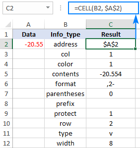
With the information you already know, you should have no difficulties with interpreting the formula results, maybe except the format type. And this leads us nicely to the next section of our tutorial.
Format codes
The below table lists the most typical values that can be returned by a CELL formula with the info_type argument set to "format".
| Format | Returned value |
| General | G |
| 0 | F0 |
| 0.00 | F2 |
| #,##0 | ,0 |
| #,##0.00 | ,2 |
| Currency with no decimal places
$#,##0 or $#,##0_);($#,##0) |
C0 |
| Currency with 2 decimal places
$#,##0.00 or $#,##0.00_);($#,##0.00) |
C2 |
| Percentage with no decimal places
0% |
P0 |
| Percentage with 2 decimal places
0.00% |
P2 |
| Scientific notation
0.00E+00 |
S2 |
| Fraction # ?/? or # ??/?? |
G |
| m/d/yy or m/d/yy h:mm or mm/dd/yy | D4 |
| d-mmm-yy or dd-mmm-yy | D1 |
| d-mmm or dd-mmm | D2 |
| mmm-yy | D3 |
| mm/dd | D5 |
| h:mm AM/PM | D7 |
| h:mm:ss AM/PM | D6 |
| h:mm | D9 |
| h:mm:ss | D8 |
For custom Excel number formats, the CELL function may return other values, and the following tips will help you to interpret them:
- The letter is usually the first letter in the format name, e.g. "G" stands for "General ", "C" for "Currency", "P" for "Percentage", "S" for "Scientific ", and "D" for "Date".
- With numbers, currencies and percentages, the digit indicates the number of displayed decimal places. For example, if the custom number format displays 3 decimal places, like 0.###, the CELL function returns "F3".
- Comma (,) is added to the beginning of the returned value if a number format has a thousands separator. For instance, for the format #,###.#### a CELL formula returns ",4" indicating that the cell is formatted as a number with 4 decimal places and a thousands separator.
- Minus sign (-) is added to the end of the returned value if the cell is formatted in color for negative values.
- Parentheses () is added to the end of the returned value if the cell is formatted with parentheses for positive or all values.
To gain more understanding of the format codes, please take a look at the results of the following formula, which is copied across column D:
=CELL("format",B3)
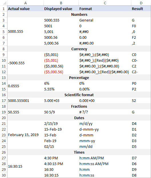
Note. If you later apply a different format to the referenced cell, you must recalculate the worksheet to update the result of a CELL formula. To recalculate the active worksheet, press Shift + F9 or use any other method described in How to recalculate Excel worksheets.
How to use the CELL function in Excel - formula examples
With the inbuilt info_types, the CELL function can return total 12 different parameters about a cell. In combination with other Excel functions, it is capable of much more. The following examples demonstrate some of the advanced capabilities.
Get address of the lookup result
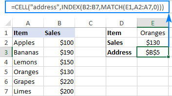
To look up a certain value in one column and return a matching value from another column, you usually use the VLOOKUP function or a more powerful INDEX MATCH combination. In case you also want to know the address of the returned value, put the Index/Match formula in the reference argument of CELL like shown below:
With the lookup value in E2, lookup range A2:A7, and return range B2:B7, the real formula goes as follows:
=CELL("address", INDEX(B2:B7, MATCH(E1,A2:A7,0)))
And returns the absolute cell reference of the lookup result:
Please note that embedding the VLOOKUP function won't work because it returns a cell value, not a reference. The INDEX function also normally displays a cell value, but it returns a cell reference underneath, which the CELL function is able to understand and process.
Make a hyperlink to the lookup result (first match)
If you wish not only to get the address of the first match, but also to jump to that match, create a hyperlink to the lookup result by using this generic formula:
In this formula, we again use the classic Index/Match combination to get the first matching value and the CELL function to extract its address. Then, we concatenate the address with the "#" character to tell HYPERLINK that the target cell is in the current sheet.
For our sample dataset, we use the same Index/Match formula as in the previous example and only need to add the desired link name, for example, this one:
=HYPERLINK("#"&CELL("address", INDEX(B2:B7, MATCH(E1,A2:A7,0))), "Go to lookup result")
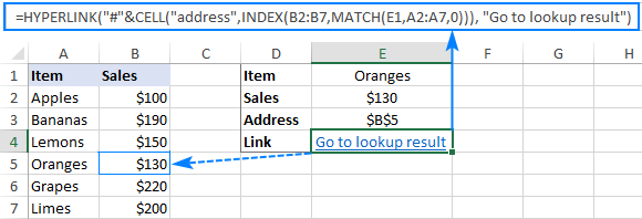
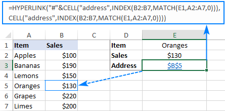
Instead to creating a hyperlink in a separate cell, you can actually turn the address into a clickable link. For this, embed the same CELL("address", INDEX(…,MATCH()) formula into the last argument of HYPERLINK:
=HYPERLINK("#"&CELL("address", INDEX(B2:B7, MATCH(E1,A2:A7,0))), CELL("address", INDEX(B2:B7, MATCH(E1,A2:A7,0))))
And make sure this lengthy formula produces a laconic and explicit result:
Get different parts of the file path
To return a full path to the workbook that contains a referenced cell, use a simple Excel CELL formula with "filename" in the info_type argument:
=CELL("filename")
This will return the file path in this format: Drive:\path\[workbook.xlsx]sheet
To return only a specific part of the path, use the SEARCH function to determine the starting position and one of the Text functions such as LEFT, RIGHT and MID to extract the required part.
Note. All of the below formulas return the address of the current workbook and worksheet, i.e. the sheet where the formula is located.
Workbook name
To output just the file name, use the following formula:
=MID(CELL("filename"), SEARCH("[", CELL("filename"))+1, SEARCH("]", CELL("filename")) - SEARCH("[", CELL("filename"))-1)

How the formula works:
The file name returned by the Excel CELL function is enclosed in square brackets, and you use the MID function to extract it.
The starting point is the position of the opening square bracket plus 1: SEARCH ("[",CELL("filename"))+1.
The number of characters to extract corresponds to the number of characters between the opening and closing brackets, which is calculated with this formula: SEARCH("]", CELL("filename")) - SEARCH("[", CELL("filename"))-1
Worksheet name
To return the sheet name, use one of the following formulas:
=RIGHT(CELL("filename"), LEN(CELL("filename")) - SEARCH("]", CELL("filename")))
or
=MID(CELL("filename"), SEARCH("]", CELL("filename"))+1, 31)

How the formulas work:
Formula 1: Working from the inside out, we calculate the number of characters in the worksheet name by subtracting the position of the closing bracket returned by SEARCH from the total path length calculated with LEN. Then, we feed this number to the RIGHT function instructing it to pull that many characters from the end of the text string returned by CELL.
Formula 2: We use the MID function to extract just the sheet name beginning with the first character after the closing bracket. The number of characters to extract is supplied as 31, which is the maximum number of characters in worksheet names allowed by the Excel UI (though Excel's xlsx file format permits up to 255 characters in sheet names).
Path to the file
This formula will bring you the file path without the workbook and sheet names:
=LEFT(CELL("filename"), SEARCH("[", CELL("filename"))-1)

How the formula works:
First, you locate the position of the opening square bracket "[" with the SEARCH function and subtract 1. This gives you the number of characters to extract. And then, you use the LEFT function to pull that many characters from the beginning of the text string returned by CELL.
Path and file name
With this formula, you can get a full path to the file including the workbook name, but without the sheet name:
=SUBSTITUTE(LEFT(CELL("filename"), SEARCH("]", CELL("filename"))-1), "[", "")

How the formula works:
The SEARCH function calculates the position of the closing square bracket, from which you subtract 1, and then get the LEFT function to extract that many characters from the beginning of the text string returned by CELL. This effectively cuts off the sheet name, but the opening square bracket remains. To get rid of it, you substitute "[" with an empty string ("").
That's how you use the CELL function in Excel. To have a closer look at the formulas discussed in this tutorial, I invite you to download our sample Workbook below. Thank you for reading and hope to see you on our blog next week!
Practice workbook for downloads
Excel CELL function -examples (.xlsx file)
 by
by
15 comments
How can I read by a formula the customised cell format?
Ex: cell = "1.002.34 CNY", cell value = 1002.34, cell format = '#.###,00 CNY'
Desired result: '#.###,00 CNY'
or something similar that I can extract the format details.
Seem not to work with =cell('format', a1)
Hi! The CELL function can't extract and display a custom number format. The article above describes the formats you can get.
Hi Team
1. I want to create a formula that finds a specific column name's address. I used =CELL("address", INDEX(FK1:FV1, MATCH(FV3,FK1:FV1,0))); so FV3 is found in range FK1:FV1. I get the correct answer $FK$1.
2. I then in a new formula, =CELL("contents",FX3), want the contents of $FK$1 (which is the answer in #1 above that is in cell FX3). I expect to get an answer that is the column name in FK1, but i get the answer $FK$1, again.
Can you please advise why i don't get the contents of FK1?
Regards
Johan
Hello! Use the INDIRECT function to create a reference based on a text value written in another cell.
=CELL("contents",INDIRECT(FX3))
I want use the function randbetwen and display the random numbers generated in another cell than the cell containing the function. I dont want vba based solution. Is there any simple trick ?
Thankfully
Prasannakumar
Hi!
I do not understand your question. Explain in more detail.
BS00492 FORM-25 MUSTER ROLL LEDGER BOOKS (50 PAGES)
BM00023 J.K.WHITE CEMENT
BM00107 BIRLA WHITE CEMENT
GC00882 WHITE PAINT
MS05757 30" 5 MICRON CATRIDGE FILTERS
BS00486 172 PAGES LONG NOTE BOOKS
GC00236 DWL 7005 CLEANING & DEWAXING OIL
PM00253 CONE COVERS 14" X 16"
PM00540 PAPER CONES PINK LAMP
PM01482 PAPER CONES BLUE DOT
PM00148 PAPER CONES VIOLET LAMP
I want to abbreviate the initials of a cell value in another cell as below
BS = Books and Stationery
BM = Building Material
PM = Packing material
please suggest me a simple method
Hello!
If I understand your task correctly, the following formula should work for you:
=IF(LEFT(A1,2)="BS","Books and Stationery",IF(LEFT(A1,2)="BM","Building Material", IF(LEFT(A1,2)="PM","Packing Material", A1 ) ) )
Hope this is what you need.
How do you determine if a User has deleted a formula in a cell and then typed in their own number? I am trying to develop a statement using a Conditional Format that would turn the cell a red color when the formula was deleted.
Thank you.
Hello Benjamin!
Please go to Conditional Formatting- > New Rule -> Use a formula to determine which cells to format and set the following formula for cell A1:
=NOT(ISFORMULA(A1))
You may refresh your knowledge about conditional formatting here https://www.ablebits.com/office-addins-blog/change-background-color-excel-based-on-cell-value/#change-color-special-cells
Hi Natalia: I have a column with 8760 rows, containing the temperatures measured every hour for the 365 days of a year (24x365=8760); I want automatize the identification of the minimum and the maximum temperature for EACH day of the year. I tried with some of your examples, but I can't see a way of doing what I need. Any suggestions? Thank you very much.
If you send me file I'll add some filters to that
How do you get excel to hyperlink to a specific phrase? For example, I have a large table of values, and I want to have another sheet with links to specific places on that document for reference. However, if someone adds a row, those hyperlinks, which are currently linked to a specific cell no longer work correctly. How could I make it so that the hyperlink either recognizes that it needs to change, or tie it to link to that specific phrase? Thanks!
Hi, is it possible to highlight birthdays within 30 days before today in google sheets. I have been looking to highlight upcoming patients birthday within 30 days before birthdate. I have a column C with birth dates that needs to be highlighted if is: Today 7 days before 30 days before The idea behind this picture is to: Acknowledge the Birthday. Send to all our patients, a birthday card. Call the patient on his birthday. Here is a link to the sheet. Thanks for the help.
Hi Jaime,
Though you didn't provide the link to your spreadsheet, here's the formula you can use in your conditional formatting to colour cells with dates within 30 days from today:
=C1-TODAY()=30
Make sure to apply the rule to your entire C column (C:C).
If you're not familiar with conditional formatting, check out this blog post of ours.