The tutorial explains the basics of Spearman correlation in a simple language and shows how to calculate the Spearman rank correlation coefficient in Excel.
When doing correlation analysis in Excel, in most cases you will deal with the Pearson correlation. But because the Pearson correlation coefficient measures only a linear relationship between two variables, it does not work for all data types - your variables may be strongly associated in a non-linear way and still have the coefficient close to zero. In such circumstances, you can do the Spearman rank correlation instead of Pearson's.
Spearman correlation - the basics
The Spearman correlation is the nonparametric version of the Pearson correlation coefficient that measure the degree of association between two variables based on their ranks.
The Pearson Product Moment Correlation tests the linear relationship between two continuous variables. Linear means a relationship when two variables change in the same direction at a constant rate.
Spearman Rank Correlation evaluates the monotonic relationship between the ranked values. In a monotonic relationship, the variables also tend to change together, but not necessarily at a constant rate.
When to do Spearman correlation
The Spearman correlation analysis is to be used in any of the following circumstances when the underlying assumptions of the Pearson correlation are not met:
- If your data exhibit a non-linear relationship or are not normally distributed.
- If at least one variable is ordinal. If your values can be placed in "first, second, third…" order, you are dealing with ordinal data.
- If there are significant outliers. Unlike the Pearson correlation, the Spearman correlation is not sensitive to outliers because it performs calculations on the ranks, so the difference between actual values does not have meaning.
For example, you can use the Spearman correlation to find the answers to the following questions:
- Are people with a higher level of education more concerned about the environment?
- Is the number of symptoms a patient has related to their willingness to take medication?
Spearman correlation coefficient
In statistics, the Spearman correlation coefficient is represented by either rs or the Greek letter ρ ("rho"), which is why it is often called Spearman's rho.
The Spearman rank correlation coefficient measures both the strength and direction of the relationship between the ranks of data. It can be any value from -1 to 1, and the closer the absolute value of the coefficient to 1, the stronger the relationship:
- 1 is a perfect positive correlation
- -1 is a perfect negative correlation
- 0 is no correlation
Spearman rank correlation formula
Depending on whether there are or there are no ties in the ranking (the same rank assigned to two or more observations), the Spearman correlation coefficient can be calculated with one of the following formulas.
If there are no tied ranks, a simpler formula will do:

Where:
- di is the difference between a pair of ranks
- n is the number of observations
To deal with tied ranks, the full version of Spearman correlation formula has to be used, which is a slightly modified version of Pearson's r:

Where:
- R(x) and R(y) are the ranks of the x and y variables
- R(x) and R(y) are the mean ranks
How to calculate Spearman correlation in Excel with CORREL function
Regrettably, Excel does not have an inbuilt function for calculating the Spearman rank correlation coefficient. However, that does not mean you will have to rack your brain with the above formulas. By manipulating Excel a bit, we can come up with a much simpler way to do Spearman correlation.
As an example, let's try to find out if our physical activity has any relation to our blood pressure. In column B, we have the number of minutes that 10 men of the same age spend daily in a gym, and in column C, we have their systolic blood pressure.
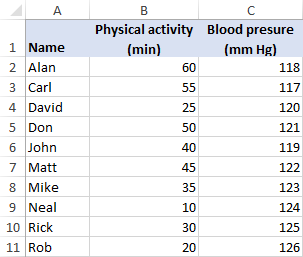
To find the Spearman correlation coefficient in Excel, perform these steps:
- Rank your data
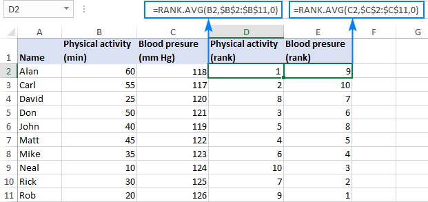
Because the Spearman correlation evaluates the associations between two variables based on their ranks, you need to rank your source data. This can be quickly done by using the Excel RANK.AVG function.
To rank the first variable (physical activity), enter the below formula in D2 and then drag it down to D11:
=RANK.AVG(B2,$B$2:$B$11,0)To rank the second variable (blood pressure), put the following formula in cell E2 and copy it down the column:
=RANK.AVG(C2,$C$2:$C$11,0)For the formulas to work correctly, please be sure to lock the ranges with absolute cell references.
At this point, your source data should look similar to this:
- Find Spearman correlation coefficient
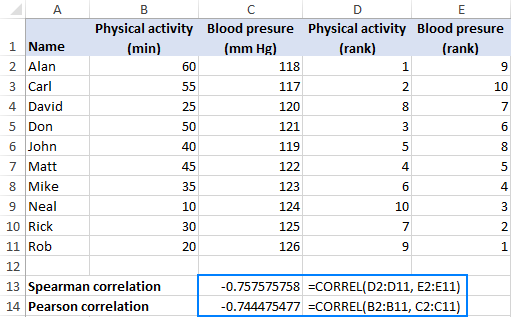
With the ranks established, we can now use the Excel CORREL function to get Spearman's rho:=CORREL(D2:D11, E2:E11)The formula returns a coefficient of -0.7576 (rounded to 4 digits), which shows a fairly strong negative correlation and allows us to conclude that the more a person exercises, the lower their blood pressure.
The Pearson correlation coefficient for the same sample (-0.7445) indicates a bit weaker correlation, but still statistically significant:
The beauty of this method is that it is quick, easy, and works regardless of whether there are ties in the ranking or not.
Calculate Spearman correlation coefficient in Excel with traditional formula
If you are not quite sure that the CORREL function has computed Spearman's rho right, you can verify the result with the traditional formula used in statistics. Here's how:
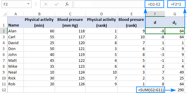
- Find the difference between each pair of ranks (d) by subtracting one rank from the other:
=D2-E2This formula goes to F2 and is then copied down the column.
- Raise each rank difference to the power of two (d2):
=F2^2This formula goes to column G.
- Add up the squared differences:
=SUM(G2:G11)This formula can go to any blank cell, G12 in our case.
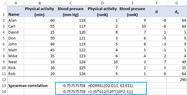
From the following screenshot, you will probably gain better understanding of the data arrangement:
- Depending on whether your data set has any tied ranks or not, use one of these formulas to calculate the Spearman correlation coefficient.
In our example, there are no ties, so we can go with a simpler formula:

With d2 equal to 290, and n (number of observations) equal to 10, the formula undergoes the following transformations:

As the result, you get -0.757575758, which perfectly agrees with the Spearman correlation coefficient calculated in the previous example.
In Microsoft Excel, the above calculations can be performed with the following equation:
=1-(6*G12/(10*(10^2-1)))
Where G12 is the sum of the squared rank differences (d2).
How to do Spearman correlation in Excel using a graph
The correlation coefficients in Excel only measure linear (Pearson) or monotonic (Spearman) relationships. However, other associations are possible. So, no matter which correlation you do, it is always a good idea to represent the relationship between the variables in a graph.
To draw a correlation graph for the ranked data, here's what you need to do:
- Calculate the ranks by using the RANK.AVG function as explained in this example.
- Select two columns with the ranks.
- Insert an XY scatter chart. For this, click the Scatter chart icon on the Inset tab, in the Chats group.
- Add a trendline to your chart. The fastest way is to click the Chart Elements button > Add Trendline….
- Display R-squared value on the chart. Double-click the trendline to open its pane, switch to the Trendline Options tab and select the Display R-squared value on chart box.
- Show more digits in the R2 value for better accuracy.
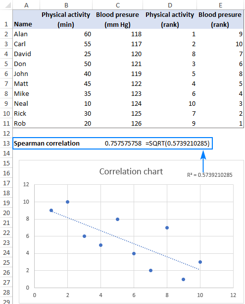
As the result, you will get a visual representation of the relationship between the ranks. Additionally, you will get the Coefficient of Determination (R2), the square root of which is the Pearson correlation coefficient (r). But because you have plotted the ranked data, this Pearson's r is nothing else but Spearman's rho.
Note. R-squared is always a positive number, hence the deduced Spearman rank correlation coefficient will also be always positive. To add an appropriate sign, just look at the line in your correlation graph - an upward slope indicates a positive correlation (plus sign) and a downward slope indicates a negative correlation (minus sign).
In our case, R2 equals 0.5739210285. Use the SQRT function to find the square root:
=SQRT(0.5739210285)
…and you will get the already familiar coefficient of 0.757575758.
The downward slope in the graph exhibits a negative correlation, so we add the minus sign and get the correct Spearman correlation coefficient of -0.757575758.
That's how you can calculate the Spearman rank correlation coefficient in Excel. To have a closer look at the examples discussed in this tutorial, you are welcome to download our sample workbook below. I thank you for reading and hope to see you on our blog next week!
Practice workbook
Spearman Rank Correlation in Excel (.xlsx file)
 by
by
19 comments
Great illustration
Dear Svetlana,
very nice example.
Is there any way to calculate a p-Val for the Spearman's correlation in Excel.
Thank you
Marc
Good examples and useful
Hi, I changed (a little) your data (in "Phisical activity" columne there are "50" twice):
Physical activity (min) Blood preasure (mm Hg)
60 118
55 117
25 120
50 121
50 119
45 122
35 123
10 124
30 125
20 126
Now i got Spearman correlation using formula: -0,803030303 and using function CORREL: -0,808514373
Why? Please help me
Because... you changed your data?
Hi, excellent examples, thank you. just one thing - you indicate a different formula is necessary if there are tied ranks (as I have in my data) but the formula is not presented. Any chance you could add this one? Thanks a lot.
Thank you for this example, it's really helpful!
I was just wondering, if one or both variables were already ordinal and not continuous, could you still do a Spearman correlation using the CORREL function as you have outlined? I'm unsure because I don't know if you would carry out the RANK.AVG function on the data if it is already ranked. Any help would be much appreciated.
great example
great explanation.
Thank you
Can you give examples if the data were to have tied ranks???
yes please
awesome!
Thank you very much for the explanation!!
There is an error in the first table with 4 columns: the first row of data is different from all other tables and gives erroneous ranking. This is just above the section called '2. Find Spearman correlation coefficient'
Hi Jeremy,
Good catch, thank you! The erroneous screenshot is replaced with the right one.
When you say "you can use the Pearson correlation to find the answers to the following questions"...did you actually mean the Spearman correlation?
Hi Vinny,
Absolutely so :) Fixed, thank you!
What if we have NA in the data, can we ignore NA and perform the sperman's correlation in excel
Excellent example
tHANK YOU, mISTER, I AM VERII GREJTFL