The tutorial explains how to use COUNTIFS and COUNTIF formulas with multiple criteria in Excel based on AND as well as OR logic. You will find a number of examples for different data types - numbers, dates, text, wildcard characters, non-blank cells and more.
Of all Excel functions, COUNTIFS and COUNTIF are probably most often mixed up because they look very much alike and both are purposed for counting cells based on the specified criteria.
The difference is that COUNTIF is designed for counting cells with a single condition in one range, whereas COUNTIFS can evaluate different criteria in the same or in different ranges. The aim of this tutorial is to demonstrate different approaches and help you choose the most efficient formula for each particular task.
Excel COUNTIFS function - syntax and usage
The Excel COUNTIFS function counts cells across multiple ranges based on one or several conditions. The function is available in Excel 365, 2021, 2019, 2016, 2013, Excel 2010, and Excel 2007, so you can use the below examples in any Excel version.
COUNTIFS syntax
The syntax of the COUNTIFS function is as follows:
- criteria_range1 (required) - defines the first range to which the first condition (criteria1) shall be applied.
- criteria1 (required) - sets the condition in the form of a number, cell reference, text string, expression or another Excel function. The criteria defines which cells shall be counted and can be expressed as 10, "<=32", A6, "sweets".
- [criteria_range2, criteria2]… (optional) - these are additional ranges and their associated criteria. You can specify up to 127 range/criteria pairs in your formulas.
In fact, you don't have to remember the syntax of the COUNTIF function by heart. Microsoft Excel will display the function's arguments as soon as you start typing; the argument you are entering at the moment is highlighted in bold.

Excel COUNTIFS - things to remember!
- You can use the COUNTIFS function in Excel to count cells in a single range with a single condition as well as in multiple ranges with multiple conditions. If the latter, only those cells that meet all of the specified conditions are counted.
- Each additional range must have the same number of rows and columns as the first range (criteria_range1 argument).
- Both contiguous and non-contiguous ranges are allowed.
- If the criteria is a reference to an empty cell, the COUNTIFS function treats it as a zero value (0).
- You can use the wildcard characters in criteria - asterisk (*) and question mark (?). See this example for full details.
How to use COUNTIFS and COUNTIF with multiple criteria in Excel
Below you will find a number of formula examples that demonstrate how to use the COUNTIFS and COUNTIF functions in Excel to evaluate multiple conditions.
How to count cells with multiple criteria (AND logic)
This scenario is the easiest one, since the COUNTIFS function in Excel is designed to count only those cells for which all of the specified conditions are TRUE. We call it the AND logic, because Excel's AND function works this way.
Formula 1. COUNTIFS formula with multiple criteria
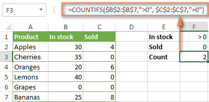
Suppose you have a product list like shown in the screenshot below. You want to get a count of items that are in stock (value in column B is greater than 0) but have not been sold yet (value is column C is equal to 0).
The task can be accomplished by using this formula:
=COUNTIFS(B2:B7,">0", C2:C7,"=0")
And the count is 2 ("Cherries" and "Lemons"):
Formula 2. COUNTIFS formula with two criteria
When you want to count items with identical criteria, you still need to supply each criteria_range / criteria pair individually.
For example, here's the right formula to count items that have 0 both in column B and column C:
=COUNTIFS($B$2:$B$7,"=0", $C$2:$C$7,"=0")
This COUNTIFS formula returns 1 because only "Grapes" have "0" value in both columns.
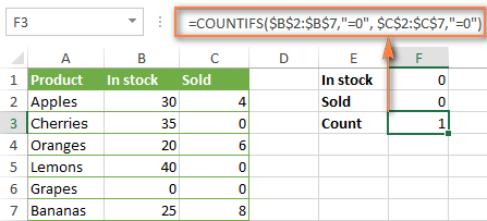
Using a simpler formula with a single criteria_range like COUNTIFS(B2:C7,"=0") would yield a different result - the total count of cells in the range B2:C7 containing a zero (which is 4 in this example).
How to count cells with multiple criteria (OR logic)
As you have seen in the above examples, counting cells that meet all of the specified criteria is easy because the COUNTIFS function is designed to work this way.
But what if you want to count cells for which at least one of the specified conditions is TRUE, i.e. based on the OR logic? Overall, there are two ways to do this - by adding up several COUNTIF formulas or using a SUM COUNTIFS formula with an array constant.
Formula 1. Add up two or more COUNTIF or COUNITFS formulas
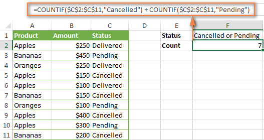
In the table below, supposing you want to count orders with the "Cancelled" and "Pending" status. To have it doen, you can simply write 2 regular Countif formulas and add up the results:
=COUNTIF($C$2:$C$11,"Cancelled") + COUNTIF($C$2:$C$11,"Pending")
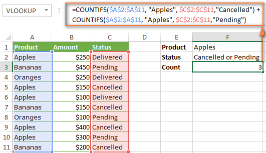
In case each of the functions is supposed to evaluate more than one condition, use COUNTIFS instead of COUNTIF. For example, to get the count of "Cancelled" and "Pending" orders for "Apples" use this formula:
=COUNTIFS($A$2:$A$11, "Apples", $C$2:$C$11,"Cancelled") + COUNTIFS($A$2:$A$11, "Apples", $C$2:$C$11,"Pending")
Formula 2. SUM COUNTIFS with an array constant
In situations when you have to evaluate a lot of criteria, the above approach is not the best way to go because your formula would grow too big in size. To perform the same calculations in a more compact formula, list all of your criteria in an array constant, and supply that array to the criteria argument of the COUNTIFS function. To get the total count, embed COUNTIFS inside the SUM function, like this:
In our sample table, to count orders with the status "Cancelled" or "Pending" or "In transit", the formula would go as follows:
=SUM(COUNTIFS($C$2:$C$11, {"cancelled", "pending", "in transit"}))
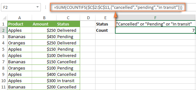
In a similar manner, you can count cells based on two or more criteria_range / criteria pairs. For instance, to get the number of "Apples" orders that are "Cancelled" or "Pending" or "In transit", use this formula:
=SUM(COUNTIFS($A$2:$A$11,"apples",$C$2:$C$11,{"cancelled","pending","in transit"}))

You can find a few more ways to count cells with OR logic in this tutorial: Excel COUNTIF and COUNTIFS with OR conditions.
How to count numbers between 2 specified numbers
By and large, COUNTIFS formulas for numbers fall into 2 categories - based on several conditions (explained in the above examples) and between the two values you specify. The latter can be accomplished in two ways - by using the COUNTIFS function or by subtracting one COUNTIF from another.
Formula 1. COUNTIFS to count cells between two numbers
To find out how many numbers between 5 and 10 (not including 5 and 10) are contained in cells C2 through C10, use this formula:
=COUNTIFS(C2:C10,">5", C2:C10,"<10")
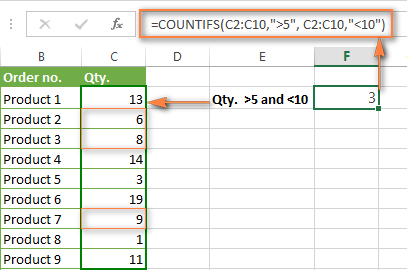
To include 5 and 10 in the count, use the "greater than or equal to" and "less than or equal to" operators:
=COUNTIFS(B2:B10,">=5", B2:B10,"<=10")
Formula 2. COUNTIF formulas to count numbers between X and Y
The same result can be achieved by subtracting one Countif formula from another. The first one counts how many numbers are greater than the lower bound value (5 in this example). The second formula returns the count of numbers that are greater than the upper bound value (10 in this case). The difference between the first and second number is the result you are looking for.
- =COUNTIF(C2:C10,">5")-COUNTIF(C2:C10,">=10") - counts how many numbers greater than 5 and less than 10 are in the range C2:C10. This formula will return the same count as shown in the screenshot above.
- =COUNTIF(C2:C10, ">=5")-COUNTIF(C2:C10, ">10") - the formula counts how many numbers between 5 and 10 are in the range C2:C10, including 5 and 10.
How to use cell references in COUNTIFS formulas
When using logical operators such as ">", "<", "<=" or ">=" together with cell references in your Excel COUNTIFS formulas, remember to enclose the operator in "double quotes" and
add an ampersand (&) before a cell reference to construct a text string.
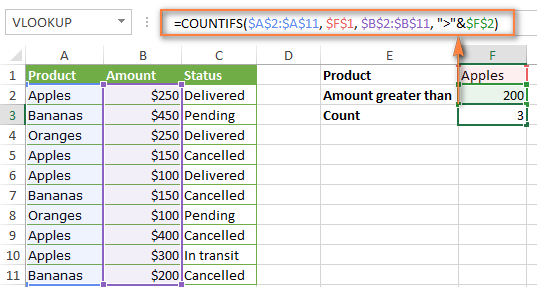
In a sample dataset below, let's count "Apples" orders with amount greater than $200. With criteria_range1 in cells A2:A11 and criteria_range2 in B2:B11, you can use this formula:
=COUNTIFS($A$2:$A$11, "Apples", $B$2:$B$11, ">200")
Or, you can input your criteria values in certain cells, say F1 and F2, and reference those cells in your formula:
=COUNTIFS($A$2:$A$11, $F$1, $B$2:$B$11, ">"&$F$2)
Please notice the use of absolute cell references both in the criteria and criteria_range arguments, which prevents the formula from being broken when copied to other cells.
For more information about the use of an ampersand in COUNTIF and COUNTIFS formulas, please see Excel COUNTIF - frequently asked questions.
How to use COUNTIFS with wildcard characters
In Excel COUNTIFS formulas, you can use the following wildcard characters:
- Question mark (?) - matches any single character, use it to count cells starting and/or ending with certain characters.
- Asterisk (*) - matches any sequence of characters, you use it to count cells containing a specified word or a character(s) as part of the cell's contents.
Tip. If you want to count cells with an actual question mark or asterisk, type a tilde (~) before an asterisk or question mark.
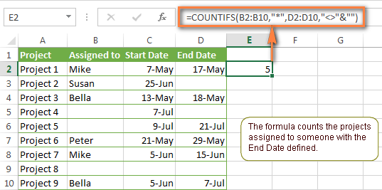
Now let's see how you can use a wildcard char in real-life COUNTIFS formulas in Excel. Suppose, you have a list of projects in column A. You wish to know how many projects are already assigned to someone, i.e. have any name in column B. And because we are learning how to use the COUNTIFS function with multiple criteria, let's add a second condition - the End Date in column D should also be set.
Here is the formula that works a treat:
=COUNTIFS(B2:B10,"*",D2:D10,"<>"&""))
Please note, you cannot use a wildcard character in the 2nd criteria because you have dates rather that text values in column D. That is why, you use the criteria that finds non-blank cells: "<>"&""
COUNTIFS and COUNTIF with multiple criteria for dates
The COUNTIFS and COUNTIF formulas you use for dates are very much similar to the above formulas for numbers.
Example 1. Count dates in a specific date range
To count the dates that fall in a certain date range, you can also use either a COUNTIFS formula with two criteria or a combination of two COUNTIF functions.
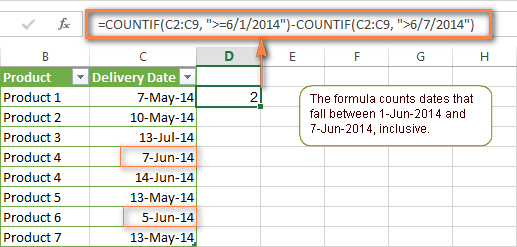
For example, the following formulas count the number of dates in cells C2 through C10 that fall between 1-Jun-2014 and 7-Jun-2014, inclusive:
=COUNTIFS(C2:C9, ">=6/1/2014", C2:C9, "<=6/7/2014")
=COUNTIF(C2:C9, ">=6/1/2014") - COUNTIF(C2:C9, ">6/7/2014")
Example 2. Count dates with multiple conditions
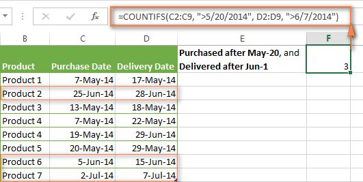
In the same manner, you can use a COUNTIFS formula to count the number of dates in different columns that meet 2 or more conditions. For instance, the below formula will find out how many products were purchased after the 20th of May and delivered after the 1st of June:
=COUNTIFS(C2:C9, ">5/1/2014", D2:D9, ">6/7/2014")
Example 3. Count dates with multiple conditions based on the current date
You can use Excel's TODAY() function in combination with COUNTIF to count dates based on the current date.
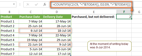
For example, the following COUNTIF formula with two ranges and two criteria will tell you how many products have already been purchased but not delivered yet.
=COUNTIFS(C2:C9, "<"&TODAY(), D2:D9, ">"&TODAY())
This formula allows for many possible variations. For instance, you can tweak it to count how many products were purchased more than a week ago and are not delivered yet:
=COUNTIFS(C2:C9, "<="&TODAY()-7, D2:D9, ">"&TODAY())
This is how you count cells with multiple criteria in Excel. I hope you will find these examples helpful. Anyway, I thank you for reading and hope to see you on our blog next week!
 by
by
1975 comments
I am trying to count rows were either column E -OR- F meet a criteria. Example.. Column A is a Truck, Column B is Trailer, I want to have a count of "1" if either the truck or trailer is red, same if both the truck and trailer are red. I only want to count if either column A -OR- Column B, but don't want to count a RED truck and RED trailer as 2. The full goal of this would be to count how many instances of each state had either a Red Truck or Trailer. Using the small subset below. I would be looking for the answer of the formula to show that CA=2 (not 3), AZ=1, etc. using the subset below:
STATE TRUCK TRAILER
---------- ---------- -----------
CA Red Blue
CA Red Red
AZ Blue Red
AZ Blue Green
I currently have a formula similar to this, but it is counting the RED Truck and the RED Trailer as 2.
=COUNTIFS(B4:B14,B2,E4:E14,"RED")+COUNTIFS(B4:B14,B2,F4:F14,"RED") get count of 1 which is correct
=COUNTIFS(B4:B14,B3,E4:E14,"RED")+COUNTIFS(B4:B14,B3,F4:F14,"RED") get count of 3 which is incorrect
I have also tried
=SUM(COUNTIFS(B4:B14,B2,E4:E14,"RED")+COUNTIFS(B4:B14,B2,F4:F14,"RED")) get count of 1 which is correct
=SUM(COUNTIFS(B4:B14,B3,E4:E14,"RED")+COUNTIFS(B4:B14,B3,F4:F14,"RED")) get count of 3 which is incorrect
B1:B14 would be the row of states, B2 is AZ, B3 is CA in the formula above.
Thanks,
WK
Hello! To avoid duplicate counts, you can use three different conditions and find the sum of the three COUNTIFS formulas:
=COUNTIFS(B4:B14,B2,E4:E14,"RED",F4:F14,"<>RED") + COUNTIFS(B4:B14,B2,E4:E14,"<>RED",F4:F14,"RED") + COUNTIFS(B4:B14,B2,E4:E14,"RED",F4:F14,"RED")
You can also use the SUMPRODUCT formula:
=SUMPRODUCT((B4:B14=B2) * (((E4:E14="red")+(F4:F14="red"))>0))
I hope it’ll be helpful.
I have in name manager a list_of_cells =$H6;$Q6;$U6;$V6.
The result of =COUNTIF(list_of_cells ;">=3") is #VALUE!
Haw can i count haw many of values in that discontinue range are greater than or equal to 3?
Hi! The COUNTIF function can only count values in a continuous range. Just count them:
=(H6>=3)+(Q6>=3)+(U6>=3)+(V6>=3)
Ty for replay,
Yes, meanwhile I used the formula =SUM($H6>=3;$Q6>=3;$U6>=3;$V6>=3).
Problem solved!
I have the following table
Platform Ticket Number Ticket Details Weight Agent
Platform1 093uf session issues 5 Agent1
Platform2 35654 session issues 5 Agent2
Platform2 768566 session issues 3 Agent1
I need the following table to be filled from the 1st table
Agent Weight Platform1 Platform2
Agent1 sum all weight of Agent1 sum all weight of platform1 for Agent1 sum all weight of platform2 for Agent1
Agent2 sum all weight of Agent2 sum all weight of platform1 for Agent2 sum all weight of platform2 for Agent2
Hi! Have you tried the methods described in this blog post? If you are not satisfied, please let me know and I will try to help you.
Here is an example formula:
=SUMIFS(E2:E10,F2:F10,"Agent1",A2:A10,"Platform1")
Hi,
can you do a countif if I have 2 columns where the result and be positive in either column?
So for example, I have a list of 100 blood donors and 2 columns of interest. One column is blood group collected on the day of donation and one where blood group was already available. The answer in either column is yes or no. I want to know the number of people who either had blood group collected on the day or it was already available. So if either column answers yes I want them to be counted but the total should not be the number of the first column plus the second it should be if the positive factor is present in either column.
I hope that makes sense, thank you for your help!
Hi! Based on the information provided, the formula could look like this:
=SUMPRODUCT(--(((C1:C20="yes") + (D1:D20="yes"))>0))
To convert TRUE and FALSE to 1 or 0, use mathematical operations (e.g., double minus --). For more information, please visit: Excel SUMPRODUCT function with multiple criteria.
Hello, we use a 'sign in' app to track when employees are working in the office, as a pose to working from home. I am trying to see how many dates have been signed in within a weekly date range for a specific person. I have used this formula =COUNTIFS(G2:G9, ">=18/03/2024", G2:G9, "=K2", G2:G9, "<=L2") it does not work. Is there a way that I can make the formula use dates in a cell instead of having to write them in. Many thanks.
Hi! Study the guidelines in the article above carefully to write the conditions in the formula correctly. Also use these instructions: COUNTIF formulas for dates. You can write the start and end date in separate cells and use references to those cells in the formula. For example:
=COUNTIFS(G2:G9, ">="&A1, G2:G9, "<="&A2, H2:H9, K2)
Further to my earlier post, I should have said that I enter the names of Goalscorers into a single cell.
You cannot do value counting on a part of a text string. Split text into separate cells. Read more: Split string by delimiter or pattern, separate text and numbers.
COUNTIFS counts every name in a text string within a cell, and does this over every row within the column, but if a name is entered twice within the same cell, it only recognises the name once in the count.
That's why I recommended separating names by cell.
You can try counting how many times a word written in D1 occurs in the text in the range A1:A10. The TEXTJOIN function combines all text into a single string. The TEXTSPLIT function creates an array of words. These words can be compared to D1 and counted as matches. I can't see your data, but maybe it will work if your Excel has these functions.
=SUM(--(TEXTSPLIT(TEXTJOIN(" ",,A1:A10),," ")=D1))
Hi, I have a football league table, and in one column, over 38 rows, I enter the names of each Goalscorer. I want to produce a list detailing how many goals each player has scored.
The COUNTIFS function works… except if a player has scored more than one goal in a game, it does not count the true total each player has scored.
Can you help?
Hi! If I understand your task correctly, try to use SUMIF or SUMIFS functions.
is there a way to add multiple words in countif function for same range row ?
Hi! To count by multiple criteria, follow the instructions above: How to use COUNTIFS and COUNTIF with multiple criteria. Or describe the problem in more detail.
Hi! I have a large amount of data with various titles, and I am trying to count the number of titles that contain certain words, while the status also being open. The original equation I had used, using OR logic: =SUM(COUNTIFS(($B:$B", {"*pile*","*extraction*","*refusal*"}, $C:$C, "Open"), seemed to work at first, but if two of the words were used in the same title, it would count it as 2. I then proceeded to just subtract all of the possible combinations using AND logic and got the following equation:
=SUM(COUNTIFS($B:$B, {"*pile*","*extraction*","*refusal*"},$C:$C, "Open")) - SUM(COUNTIFS($B:$B, "*pile*", $B:$B, "*extraction*", $C:$C, "Open")) - SUM(COUNTIFS($B:$B, "*pile*", $B:$B, "*refusal*", $C:$C, "Open")) - SUM(COUNTIFS($B:$B, "*extraction*", $B:$B, "*refusal*", $C:$C, "Open")) - SUM(COUNTIFS($B:$B, "*pile*", $B:$B, "*extraction*", $B:$B, "*refusal*", $C:$C, "Open"))
This equation works, but if I wish to add more "key words" to look for, the formula just gets very large and confusing.
So my first question is: is there a way to count with a bunch of key words, while preventing them from double counting the ones that remain in the same cell. - Within the data each line contains a unique ID number, I thought perhaps this could be used to prevent double counting, but I wasn't sure how to implement it.
Secondly, I was wondering how I would format the equation if I wanted each of the words (pile, refusal, extraction), to be referenced from a cell. I have tried using ampersands and many quotation marks to format it, but I can't seem to get it to work.
Please let me know!
Hi! If I understand your task correctly, the following formula should work for you:
=SUMPRODUCT(--((ISNUMBER(SEARCH("pile",B1:B10)) + ISNUMBER(SEARCH("extraction",B1:B10)) + ISNUMBER(SEARCH("refusal",B1:B10)))>0))
For more information, please read: How to find substring in Excel
Can I put the results of 2 Countifs in the same Cell? I'll try to show what I'm lookin for. I've tried 2 Countif equations in the cell, each by itself works. But both together, but together do not. I'm sure I'm messing up the separator between the 2. This is my Countifs =COUNTIF($H3:$H50,"Blue")& " Blue". Then another for Red.
2 Blue, 1 Red (This line in 1 Cell as a result of 2 Countifs)
Blue
Yellow
Blue
Green
Red
Hope this is enough info. Thank you.
Hi! You can combine the results of multiple formulas into a single text string using the & operator or CONCATENATE function.
=COUNTIF($H3:$H50,"Blue")& " Blue "&COUNTIF($H3:$H50,"Red")& " Red"
Read more: CONCATENATE in Excel: combine text strings, cells and columns.
Brilliant, thank you. Worked like a charm. I feel dumb because I think I used every symbol except the most obvious one.
Hello! I have a range of dates I am looking at, and for those dates, one of two options will occur. I am trying to sum option A and option B by month. I have tried a COUNTIF similar to index match, but Excel is multiplying the data,
I am looking to count up the number of instances that option A and option B occur in February, then March, then so on; and show a comparison between the two by month.
Thanks for any help you can give!
Hi! Unfortunately, this information is not enough to understand what you need. Do you want to calculate OR logic or AND logic? Have you tried any of the methods described in this blog post? If they don't work for you, give an example of the source data and the expected result.
CL 8 JH 6 YYY 7 BM 4 AA 3
CL 8 JH 6 YYY 7 BM 4 YYY 3
LC 6 GB 8 AA 7 BM 4 YYY 3
LC 6 GB 8 AA 7 BM 4 GW 3
LC 6 GB 8 AA 7 BM 4 GW 3
LC 6 GB 8 YYY 7 BM 4 GW 3
how do i calculate sum of"CL" periods
Hi! You can calculate the sum by condition using the SUMIF function. Read more: How to use SUMIF function in Excel with formula examples.
Can someone help I dont know how to implement the Countifs formula is the sheet e.g. Column A2 has date B2 has Reference number Column C2:C5 has multiple items for that reference number. The next Reference number start from B6 and so on. I want count all reference based on date column. I want to make summary on weekly basis. The Column A2:A5 has same date uses it for SUMIFS so I can not leave it empty.
Hi! From your description, it is difficult to have a full understanding of your task. I’ll try to guess and offer you the following guide: Count unique values with criteria. If this is not what you intended to calculate, it would be helpful if you could provide an example of the source data and the desired result.
A B C D E F G H
Date Reference Items Value
05/02/2024 AA12 A £60 FEBRUARY
05/02/2024 C £40
05/02/2024 D £40 Weekly Breakdown Value Count
05/02/2024 F £20 01/02/2024 SUMIFS ?
05/02/2024 F £6.95 05/02/2024 SUMIFS ?
12/02/2024 SUMIFS ?
08/02/2024 BB13 da £129.00 19/02/2024 SUMIFS ?
08/02/2024 ss £18.00 26/02/2024 SUMIFS ?
08/02/2024 sa £14.00 Total XXXX 0
16/02/2024 CC14 aa £40.00
16/02/2024 ss £40.00
16/02/2024 sss £40.00
16/02/2024 asa £50.00
16/02/2024 assd £14.00
16/02/2024 afsaf £6.00
My sheet is like this I want to make weekly report (Column F to H) based on data on left side from Column A to D. For Values sum I used SUMIFS with Date as criteria in Column G. I want to Count The Column B reference based on date as criteria. So the count of each week comes ups in summary report based on data in Column A and B.
A....................B..............................C................D
Date..............Reference.............Items..........Value
05/02/2024..............AA12..............A...........£60.00
05/02/2024.....................................C........... £40.00
05/02/2024.....................................D...........£40.00
05/02/2024.....................................F........... £20.00
05/02/2024.....................................F........... £6.95
12/02/2024..............BB13..............A...........£60.00
12/02/2024.....................................C........... £40.00
12/02/2024.....................................D...........£40.00
19/02/2024..............CC14..............A...........£60.00
19/02/2024.....................................C........... £40.00
19/02/2024.....................................D...........£40.00
Summary Table
F........................................G......................H
Weekly Breakdown.........Value.............Count
01/02/2024.....................SUMIFS ...........?
05/02/2024.....................SUMIFS ............?
12/02/2024.....................SUMIFS ............?
19/02/2024....................SUMIFS ............?
26/02/2024....................SUMIFS..............?
My sheet is like this I want to make a weekly report (Columns F to H) based on data in Columns A to D. For Values sum I used SUMIFS with Date as criteria in Column G. I want to Count The Column B reference based on date as criteria. So the count of each week comes ups in a summary report based on data in Columns A and B.
Hi! If I understood the question correctly, all the information you need is in the article above. Also pay attention to the instructions: Using Excel COUNTIF function with dates. For example:
=COUNTIFS(B2:B10,""&"",A2:A10,">="&DATE(2024,2,1),A2:A10,"<="&DATE(2024,2,5))
Your summary table does not have an example of the desired result and does not match the description of the question. So if I don't guess, ask precisely.
When I apply this formula it gives me the count of both A and B columns, but I only want to count column B. In the above case, it should be 1 in the first week.
The COUNTIFS formula counts the values in one column B that match the conditions in column A. Read the article above carefully. And explain what you want to do.
I am working with a sheet where I have drop down menu with three options, poficient, accomplished, developing, needs assistance and want to count only profient and accomplished and divide them by the number of row
so i have 4 rows and but what to count only proficient and accomplish ratings and then /4 rows to get an average out of 100 point
Hi! You can count the number of values for each variant using the COUNTIF function. You can count the total number of values using the COUNTA function. You can count the number of rows in the range of values using the ROWS function. I cannot give you a more precise answer because your explanations are not very clear.
I am trying to use a formula to count the number of cells in a table from a drop down field which fall into two dates in a table. Does that make sense?
So quarterly or monthly data range measuring the number of referrals from a specific Area:
Referral area:
WARD x
WARD y
WARD Z
( Table data collated will have date of referral )
Hi! Have you tried the ways described in this blog post? If they don’t work for you, then please describe your task in detail. As it's currently written, it's hard to tell exactly what you're asking.
I have tried but unable to make it work for me. Forgive my basic excel knowledge but if i had a source table where there was a date of entry for every row added basic example
Apple 01.04.2024
Apple 01.02.2024
Pear 03.02.2024
Bannana04.02.2024
Pear 01.03.2024
Apple 05.02.2024
I need a formula to count the entries for apple and pears between monthly and Q1 dates
Is that any clearer i can count the number of entries and the amount between two dates but not both
Hi! Pay attention to the following paragraph of the article above: Count cells with multiple criteria (OR logic). Here is a guide to the counting of dates that are within a certain interval: COUNTIF formulas for dates.
The formula might look like this:
=COUNTIFS(A1:A6,"apple",B1:B6,">="&"2024-01-01",B1:B6,"<"&"2024-04-01") + COUNTIFS(A1:A6,"pear",B1:B6,">="&"2024-01-01",B1:B6,"<"&"2024-04-01")
Thank you for the detailed tutorial. It was very helpful in understanding how these formulas function.
Regarding this example:
Formula 2. COUNTIFS formula with two criteria
When you want to count items with identical criteria, you still need to supply each criteria_range / criteria pair individually.
For example, here's the right formula to count items that have 0 both in column B and column C:
=COUNTIFS($B$2:$B$7,"=0", $C$2:$C$7,"=0")
This COUNTIFS formula returns 1 because only "Grapes" have "0" value in both columns.
How would I be able to apply this if I need to count blanks?
I tried using the following formula, but it did not work and appears to have given me ALL the blanks instead of the blanks that meet the first countifs criteria.
=COUNTIFS ($D:$D,$B5,$U:$U,$F$2) + COUNTBLANK ($S:$S) <-- this version gave me a ridiculous number, assuming it went to infinity.
So then I went to go see what my current row count was and changed it to $S1:$S855, but it still returned the incorrect count.
Is there a way to get it to countifs, then based off of those matches, if column S has blanks, to spit out a total?
Is there a way to do it without having to input row count each time?
Thank you for your help!
Hi! If I understand your task correctly, try the following formula:
=COUNTIFS($D:$D,$B5,$U:$U,$F$2,$S:$S,"")
Hi
I want to select my source from a different worksheet for my countifs formula, it is not working. It works well when I do it in the same worksheet.
How do I go about it?
Hi! If I understand your task correctly, the following tutorial should help: Excel reference to another sheet or workbook (external reference).
is there a way to count multiple ranges (a variety from three different columns) for two criteria's?
Hi! The COUNTIF function counts values in only one range. To calculate values in several data ranges, look at the SUMPRODUCT function. Read more: Excel SUMPRODUCT function with multiple criteria.
Hi Dear, I am having a hard time to find out the formula, I have 3 range references, 1st range I want to count the not equal to values, and the other 2 ranges I want to count with equal criteria but I could’nt get the actual counts after I validate from my table source
Hi! Unfortunately, this information is not enough to understand what you need. To understand what you want to do, give an example of the source data and the expected result.
Kindly help with formula to count only visible cells with values greater than zero
Hi! The COUNTIF function counts all cells. It does not matter if they are hidden or visible. You can use the Excel filter to hide cells less than zero. Then count the visible cells in the column using the AGGREGATE function. For example:
=AGGREGATE(2,5,C:C)
Is there anyway to use wildcard along with Cell references?
for eg.
Column A has the base words like A1 = 'Rice", A2 ="Noodle" etc and I want to find the number of cells in Column B which has data like fried rice, brown rice, flat noodles, noodle soup etc.
something like COUNTIF(B:B,*A1*)
Hi! You can use wildcards to find and count partial matches using the COUNTIF and COUNTIFS functions. Try to follow the recommendations from this article: COUNTIF formulas with wildcard characters (partial match).
=COUNTIFS('Document Master'!$H$11:$H$378,"Philippe MURPHY",'Document Master'!$P$11:$P$378,">="&H72,'Document Master'!$P$11:$P$378,"<="&EOMONTH(H72,0),'Document Master'!$Q$11:$Q$378,"Approved")
This formula is working, however, I want to count also not only "Approved" documents but also "For information only" documents.
How do i do that?
Hi! Please re-check the article above since it covers your task. Read following paragraph: Count cells with multiple criteria (OR logic). I can't recommend you a formula that contains unique references to your data that I don't have.
Hello,
I have cells A1,A3,A5,A7 - I need to find out if they add up to 40 - if they dont for it to be a 0 and if they do to be the difference.
How would I put that into a formula please.
So if they added up to 28 the answer woudl be 0. But if they added up to 48 the difference woudl be 8. Thank you so much.
Hi! You can find the difference and select the maximum value using the MAX formula. You can also use the IF function as shown in the examples below.
=MAX(0,SUM(A1,A3,A5,A7)-40)
=IF(SUM(A1,A3,A5,A7)-40>0,SUM(A1,A3,A5,A7)-40,0)
Thank you so much.
best wishes,
Nina
What about if I whant to count a cell that contains this data "Proj 34d Late", but in the other cells i can have "Late", "On Time", "Proj 0d On Time", and "Proj 5d Earlier"
Hi! Pay attention to the following paragraph of the article above: Count cells with multiple criteria (OR logic). You can also count all cells that have a certain word in them. For example:
=SUMPRODUCT(--(ISNUMBER(SEARCH("late",A1:A10))))
For more information, please read: How to find substring in Excel
Happy New Year to all!
Hi Alex! This formula works, but running with the issue is also counting when in the cell I have "Proj. 268 LATE" with the "48d LATE". How I can exclude counting when there is a projection in the future "Proj. #d LATE" in the A1:A#10, and only count the present milestones that are Late - "#d LATE"? Appreciate the help once again. I'm learning here. Thanks.
I gave you a link to the instructions for you to read. To look for a different text string, just change it in the formula. Instead of "late" it's "d late".
hi
i have problem with countifs :
when i type this formul
=countifs(Database!D2:D100;A5;Database!D2:D100;"="&A2)
It gives me the correct answer
But when type this formul
=countifs(Database!D2:D100;A5;Database!D2:D100;"<="&A2)
it give me 0
That is the wrong answer.
How should I modify the formula?
Hi! I can't check your formula because I don't have your data.
How can I send you an example of my data?
thank you
Sorry, we don't work with user data. You can try writing an example of the data in a blog post.
Thank you, I think I explained it wrong. I want to find the estimate of numbers smaller than a certain number for me, for example ?=> 1400
،I write this number (1400) in the cell A2
،The answer should be obtained from table2 in the sheet i called DataBase
Look for the example formulas here: COUNTIF function in Excel - count if not blank, greater than, duplicate or unique. To correctly create a table reference, use these instructions: Structured reference in Excel tables.
Hi,
I have COUNTIF working in my spreadsheet to count how many projects a person is on (example: John Smith can be on 4 different projects at 25%) however, if John Smith has "AL" (annual leave) instead of a percentage of work on that project for the week how would I display "AL" instead of the sum of 4 projects to give a high level overview that the person is on annual leave?
I will need this to also reflect for Parental Leave (PL)
Hi! If I understand your task correctly, the following formula should work for you:
=IF(COUNTIFS(A1:A10,"John Smith",B1:B10,"AL"),"AL",COUNTIF(A1:A10,"John Smith"))
Hi, How to flashfill or autofill the COUNTIFS
Hi! Maybe this guide will be helpful: Excel - autofill formulas.
Hello, how can i count data with COUNTIF that have an operator like "<IDR 1000" as text, not as command/formula? is it included in wildcard type?
Hi! The expression "
hi.
i have problem
i want, Count the number of uneven numbers, using the countifs function in two different sheets
this formula i use
=countifs(table2[name];A5;table2[number];"<="&A2)
table2 in another sheet i called MyDataBase
cell A2 is also the place where I write my number
thanks for help me
Hi! You cannot use the COUNTIFS function to count odd numbers because COUNTIFS cannot use other functions as a range or criteria argument. This SUMPRODUCT formula counts the number of odd numbers in a range using the ODD function.
=SUMPRODUCT(--(A1:A10=ODD(A1:A10)))